Vectors, Scalars and Vector Spaces
In 2017, researchers at Google Brain published Attention Is All You Need, introducing the Transformer architecture that now underlies GPT-4, Gemini, and virtually every state-of-the-art language model. At the heart of that architecture (and of every neural network, recommendation system, and computer vision model) is a deceptively simple object: the vector.
When a language model reads the word “bank”, it doesn’t see a string. It sees a vector in a 4096-dimensional space where “bank (financial)” and “bank (riverbank)” occupy measurably different regions. When a search engine decides that your query matches a document, it is computing an angle between two vectors. When a neural network learns, it is moving vectors through space in response to a gradient, itself a vector.
This article builds your working foundation for all of that. By the end, you will be able to:
- Formally define vectors, scalars, and vector spaces, and explain why the axioms matter.
- Compute norms, dot products, and inter-vector angles both by hand and in NumPy.
- Reason geometrically about high-dimensional data, a non-negotiable skill for Machine Learning research.
- Read a research paper that uses vector notation without losing the thread.
No fluff, let’s start.
Prerequisites
Before reading this article, you should be comfortable with:
- High school algebra: variables, functions, the coordinate plane.
- Python basics: lists, loops, functions, importing libraries.
- Basic calculus intuition (helpful but not required): the idea that a derivative points in the direction of steepest increase.
Intuition first
The programmer’s analogy: vectors as typed arrays with geometric soul
As a developer, you’ve used arrays your whole career. A Python list [3.0, -1.5, 7.2] stores three numbers. A vector is superficially the same thing, but with a crucial additional structure: position in space and the geometry that connects positions.
Think of it this way. If you have two dictionaries in Python:
user_A = {"age": 28, "purchase_freq": 5, "avg_spend": 120.0}
user_B = {"age": 29, "purchase_freq": 6, "avg_spend": 115.0}
As dictionaries, they’re just data blobs. You can read values, but “how similar are these users?” is not a question the dictionary can answer natively. Now convert them to vectors:
A = [28, 5, 120.0]
B = [29, 6, 115.0]
Suddenly you have geometry. You can measure the distance between them, the angle they form relative to the origin, and whether one is a scaled version of another. This is the leap vectors make over plain arrays: they live in a space equipped with rules for measuring, comparing, and transforming.
Geometric picture: vectors as arrows
Picture a standard 2D coordinate system. The vector is an arrow starting at the origin and ending at the point . Two things define it completely: its magnitude (how long the arrow is) and its direction (which way it points).
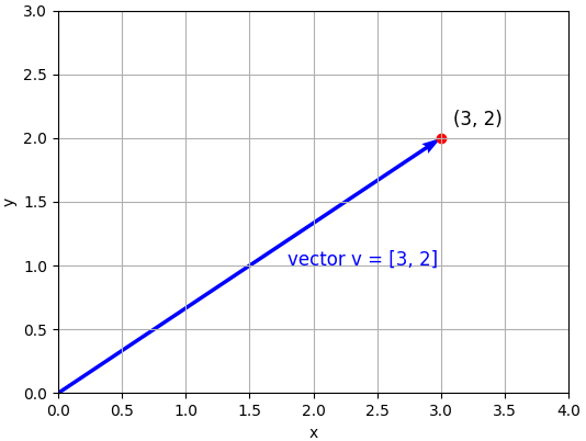
Visual representation of a two-dimension vector
This geometric interpretation is not just visual sugar. In Machine Learning, a data point (a row in your dataset) is a vector, it’s an arrow in feature space. Two similar data points are arrows pointing in roughly the same direction. An outlier is an arrow pointing somewhere unexpected. Dimensionality reduction (PCA, UMAP) is the art of finding a lower-dimensional space where those arrows still tell roughly the same story.
Scalars: the simplest case
A scalar is just a single number, no direction, no components. Temperature, loss value, learning rate: all scalars. When you multiply a vector by a scalar, you stretch or shrink the arrow without rotating it:
Same direction vector, twice as long.
2 x [3, 2] = [6, 4]Same direction vector, flipped (180°).
-1 x [3, 2] = [-3, -2]This operation, scalar multiplication, is one of the two foundational operations that define a vector space.
Mathematical derivation
Formal definitions
Scalar
An element of a field , for our purposes, a real number or complex number . Denoted with standard italics and usually greek characters: , , .
Vector
An ordered tuple of scalars from . An -dimensional real vector is an element of the space :
Vectorial space
A set of vectors over a field , equipped with two operations, for which it is closed.
Vector addition: for all . Internal operation with the following properties:
- Associativity: .
- Commutativity: .
- Identity element: there exists a vector , called zero vector, such that for all .
- Inverse element: for all , there exist an element such as .
Scalar multiplication: for all . External operation with the following properties:
- Associativity: .
- Identity element: there exists an scalar , such as para todo .
- Distributivity of scalar multiplication with respect to vector addition: For any scalar , it is true that for all .
- Distributivity of scalar multiplication with respect to scalars addition: For any two scalars and , it is true that for every .
What does it mean that the vector space is closed for those operations?
It means that they produce results that are in the same vector space.
- If and then .
- For any scalar and vector , then .
Vector addition
Given and :
Vector norms
The norm of a vector measures its length. The most common is the Euclidean norm ( norm):
The general family is the norm:
Two special cases appear constantly in Machine Learning (ML):
norm (Manhattan):
Used in LASSO regularisation because it induces sparsity, it penalizes any non-zero component equally.
norm (max norm):
Useful when you care about the single largest activation.
To dig more about Vector norms, check this Wikipedia article.
The dot product
The dot product (inner product) of two vectors is:
The dot product of a vector and itself results in its magnitude squared.
The angle between vectors
Here is where geometry and algebra merge beautifully. From Euclidean geometry, the Law of Cosines states that for a triangle with sides , , and angle opposite side :
Now apply this to vectors. Let and be two vectors. The third side of the triangle they form is .
Substituting , , :
Expanding the left side:
Cancelling and from both sides:
Dividing both sides by (assuming neither vector is zero):
Key interpretations:
- (): vectors point in the same direction (identical topics in a document embedding).
- (): vectors are orthogonal, completely unrelated.
- (): vectors point in opposite directions (antonyms in a well-trained embedding space).
In the original Word2Vec paper (Mikolov et al., 2013), the famous analogy:
works precisely because of this geometry. Semantic relationships are encoded as directions in vector space, and finding queen means finding the vector whose cosine similarity to the query vector is maximized. Every modern embedding model (BERT, GPT, sentence-transformers) inherits this geometric philosophy. Next time you read something about word representation in vector spaces, remember they are talking about the same geometry we just derived.
The cross product
The dot product takes two vectors and returns a scalar. The cross product takes two vectors in and returns a vector, one that is perpendicular to both inputs. It is defined only in three (and seven) dimensions, which makes it more geometrically specialised than the dot product.
Given and , the cross product is computed by expanding the following symbolic determinant:
Expanding along the first row:
Two geometric facts define the cross product completely:
Direction: is always orthogonal to both and . You can verify this directly: and . The orientation follows the right-hand rule: curl the fingers of your right hand from toward , and your thumb points in the direction of .
Magnitude: The length of the result equals the area of the parallelogram spanned by and , which can be expressed as:
Key algebraic property, anticommutativity:
Swapping the order flips the sign and the direction. This means the cross product is not commutative, unlike the dot product.
Python implementation
Let’s implement everything from scratch, first in pure Python, then verify with NumPy.
Code
"""
Course:  Artificial Intelligence
Módulo:  Linear Algebra
Article: Vectors, Scalars & Vector Spaces

Pure Python implementation
Python 3.10+
"""
import math
from typing import List


###################
# Vector operations
###################

def vector_add(u: List[float], v: List[float]) -> List[float]:
    """
    Add two vectors element-wise.
    Requires: u and v have the same dimension.
    """
    assert len(u) == len(v), f"Dimension mismatch: {len(u)} vs {len(v)}"
    return [u_i + v_i for u_i, v_i in zip(u, v)]


def scalar_multiply(alpha: float, v: List[float]) -> List[float]:
    """
    Multiply a vector by a scalar.
    Stretches/shrinks the arrow; negative alpha flips its direction.
    """
    return [alpha * v_i for v_i in v]


def l2_norm(v: List[float]) -> float:
    """
    Euclidean (L2) norm: the geometric length of vector v.
    """
    return math.sqrt(sum(v_i ** 2 for v_i in v))


def l1_norm(v: List[float]) -> float:
    """
    Manhattan (L1) norm: sum of absolute values.
    Sparsity-inducing, used in LASSO regularization.
    """
    return sum(abs(v_i) for v_i in v)


def dot_product(u: List[float], v: List[float]) -> float:
    """
    Dot product: sum of element-wise products.
    Returns a scalar measuring how much u and v 'align'.
    Requires: u and v have the same dimension.
    """
    assert len(u) == len(v), f"Dimension mismatch: {len(u)} vs {len(v)}"
    return sum(u_i * v_i for u_i, v_i in zip(u, v))


def cosine_similarity(u: List[float], v: List[float]) -> float:
    """
    Cosine similarity: dot(u,v) / (||u|| * ||v||).
    Returns a value in [-1, 1].
      1.0  -> identical direction (maximally similar)
      0.0  -> orthogonal (unrelated)
     -1.0  -> opposite direction (maximally dissimilar)
    """
    norm_u = l2_norm(u)
    norm_v = l2_norm(v)
    # Guard against division by zero (zero vector has no direction)
    if norm_u == 0 or norm_v == 0:
        raise ValueError("Cosine similarity undefined for zero vectors.")
    return dot_product(u, v) / (norm_u * norm_v)


def angle_between(u: List[float], v: List[float], degrees: bool = True) -> float:
    """
    Angle between two vectors in radians or degrees.
    Uses: theta = arccos(cosine_similarity(u, v))
    Clamp to [-1, 1] first to guard against floating-point errors
    that push cos slightly outside the valid domain of arccos.
    """
    cos_theta = cosine_similarity(u, v)
    cos_theta = max(-1.0, min(1.0, cos_theta))  # numerical clamp
    theta_rad = math.acos(cos_theta)
    return math.degrees(theta_rad) if degrees else theta_rad


def normalize(v: List[float]) -> List[float]:
    """
    Return the unit vector (length 1) pointing in the same direction as v.
    Formula: v_hat = v / ||v||
    Unit vectors are useful when you care about DIRECTION, not magnitude.
    """
    norm = l2_norm(v)
    if norm == 0:
        raise ValueError("Cannot normalize the zero vector.")
    return [v_i / norm for v_i in v]


#########
# Example
#########

if __name__ == "__main__":
    # Two 3-dimensional vectors, imagine these as two user embeddings
    u = [1.0, 2.0, 3.0]
    v = [4.0, 0.0, -1.0]

    print("==================================")
    print("Vector Operations with pure Python")
    print("==================================")
    print(f"u = {u}")
    print(f"v = {v}")

    print(f"Addition (u + v)        -> {vector_add(u, v)}")
    print(f"Scalar multiply (2 * u) -> {scalar_multiply(2.0, u)}")
    print(f"L2 norm of u (||u||₂)   -> {l2_norm(u):.4f}")
    print(f"L1 norm of u (||u||₁)   -> {l1_norm(u):.4f}")
    print(f"Dot product (u · v)     -> {dot_product(u, v):.4f}")
    print(f"Cosine similarity       -> {cosine_similarity(u, v):.4f}")
    print(f"Angle between u, v.     -> {angle_between(u, v):.2f}°")
    print(f"Unit vector of u (û)    -> {[round(x, 4) for x in normalize(u)]}")
    u_hat = normalize(u)
    print(f"Verify `||û||₂ = 1`     -> {l2_norm(u_hat):.6f}")

    print("=============================")
    print("Semantic similarity mini-demo")
    print("=============================")
    print("In real NLP, these would be word embeddings. Here we illustrate")
    print("the principle with handcrafted feature vectors.")
    print("Features: [royalty_score, masculinity, age, power]")

    king = [0.9, 0.9, 0.8, 0.9]
    queen = [0.9, 0.1, 0.8, 0.9]
    man = [0.0, 0.9, 0.5, 0.4]
    woman = [0.0, 0.1, 0.5, 0.4]
    print(f"king  = {king}")
    print(f"queen = {queen}")
    print(f"man   = {man}")
    print(f"woman = {woman}")

    print("The famous analogy: king - man + woman ≈ queen")
    analogy_vec = vector_add(
        vector_add(king, scalar_multiply(-1.0, man)),
        woman
    )
    sim_to_queen = cosine_similarity(analogy_vec, queen)
    sim_to_king = cosine_similarity(analogy_vec, king)

    print(f"king − man + woman -> {[round(x,2) for x in analogy_vec]}")
    print(f"Cosine similarity to 'queen': {sim_to_queen:.4f}")
    print(f"Cosine similarity to 'king':  {sim_to_king:.4f}")
    print("==> The analogy vector is closer to 'queen' than 'king'.")
Output
>  python vector_pure_python.en.py
==================================
Vector Operations with pure Python
==================================
u = [1.0, 2.0, 3.0]
v = [4.0, 0.0, -1.0]
Addition (u + v)        -> [5.0, 2.0, 2.0]
Scalar multiply (2 * u) -> [2.0, 4.0, 6.0]
L2 norm of u (||u||₂)   -> 3.7417
L1 norm of u (||u||₁)   -> 6.0000
Dot product (u · v)     -> 1.0000
Cosine similarity       -> 0.0648
Angle between u, v.     -> 86.28°
Unit vector of u (û)    -> [0.2673, 0.5345, 0.8018]
Verify `||û||₂ = 1`     -> 1.000000
=============================
Semantic similarity mini-demo
=============================
In real NLP, these would be word embeddings. Here we illustrate
the principle with handcrafted feature vectors.
Features: [royalty_score, masculinity, age, power]
king  = [0.9, 0.9, 0.8, 0.9]
queen = [0.9, 0.1, 0.8, 0.9]
man   = [0.0, 0.9, 0.5, 0.4]
woman = [0.0, 0.1, 0.5, 0.4]
The famous analogy: king - man + woman ≈ queen
king − man + woman -> [0.9, 0.1, 0.8, 0.9]
Cosine similarity to 'queen': 1.0000
Cosine similarity to 'king':  0.8902
==> The analogy vector is closer to 'queen' than 'king'.Machine Learning and AI perspective
Vectors are not a preliminary concept you’ll graduate from, they are the lingua franca of modern AI research. Here are three ways they appear in the context of Artificial Intelligence and Machine Learning.
Embedding spaces and representation learning. Every modern deep learning model learns to represent inputs as vectors. The Transformer’s token embeddings described in the Attention Is All You Need paper are vectors in (typically between 512 and 4096 dimensions). The entire training process can be viewed as optimizing the geometry of these vectors so that semantically similar inputs cluster together. Research on contrastive learning explicitly frames the learning objective in terms of pushing similar sample vectors together and dissimilar sample vectors apart in embedding space.
Retrieval-Augmented Generation (RAG) and vector databases. With the explosion of LLMs, a major applied-research direction is efficient nearest-neighbour search over billions of vectors. In the paper, Retrieval-Augmented Generation for Knowledge-Intensive NLP Tasks, Lewis et al. showed that augmenting generation with retrieved document vectors dramatically improves factuality. The entire retrieval step is cosine similarity search, the formula we saw before.
Dimensionality. The geometry of high-dimensional spaces is deeply counter-intuitive, a phenomenon called the curse of dimensionality. In very high dimensions, almost all pairs of vectors become nearly orthogonal (), which can degrade cosine similarity as a meaningful metric. Understanding when cosine similarity breaks down and what geometric alternatives exist (hyperbolic spaces, Riemannian manifolds) is an active research area. If this interests you, look up Poincaré Embeddings.
Common pitfalls and debugging
Forgetting to normalize before computing cosine similarity, and when NOT to. Cosine similarity measures direction only, discarding magnitude. If two documents are similar but one is ten times longer, cosine similarity ignores the length difference. Sometimes that’s a bug (when magnitude matters), sometimes a feature (sentiment classification where you want topic, not verbosity). Always ask: should magnitude matter here? If yes, use Euclidean distance instead.
Dimension mismatch silently producing wrong results. In NumPy,
np.dot(u, v)will raise an error if dimensions don’t match for 1D arrays, but with 2D arrays (matrices), NumPy may broadcast in ways that give a result with the wrong shape. Always.assert u.shape == v.shapebefore dot products in research code, or usenp.einsumwith explicit index notation for clarity.The zero-vector edge case.
cosine_similarity([0,0,0], [1,2,3])is mathematically undefined (you’re dividing by zero). In production systems that compute embeddings, a zero vector usually signals a bug upstream: an empty input, a bad tokenisation, or a collapsed network layer. If you seeNaNlosses, check your embedding norms first.Floating-point precision in
arccos. Due to floating-point arithmetic, dot products can occasionally yield cosine values slightly outside (e.g.,1.0000000002). Passing this directly tomath.acos()raises aValueError. Always clamp:cos_theta = max(-1.0, min(1.0, cos_theta))before callingarccos.Confusing and regularisation effects. regularisation (weight decay) shrinks all weights proportionally, it never drives weights exactly to zero. regularisation does drive weights to zero, creating sparse models. This is a direct consequence of the geometry of vs norm balls. Choosing the wrong regulariser is a common source of models that are either too dense (wasted computation) or not sparse enough (poor interpretability).
Summary and what’s next
Key takeaways from this article:
- A vector is an ordered tuple of scalars that lives in a geometric space, it has both magnitude and direction.
- A vector space is defined by closure under addition and scalar multiplication, this is why linear operations in neural networks are so well-behaved.
- The norm measures Euclidean length. The norm measures Manhattan distance and promotes sparsity.
- The dot product () measures alignment. Dividing by both norms gives cosine similarity, the angle-based similarity metric at the core of retrieval, embeddings, and attention mechanisms.
- The formula is derived from the Law of Cosines, it’s not arbitrary, it’s geometry.
- High-dimensional vectors are the language in which all of modern Machine Learning is written. Fluency here compounds across every future topic.
Coming up in (Matrices & Linear Transformations): We generalize from single vectors to collections of vectors, introduce matrices as functions that transform vector spaces, and derive the rules of matrix multiplication from first principles. You’ll see exactly why a fully-connected neural network layer is nothing more than a matrix multiplication followed by a nonlinearity.
Cheers for making it this far! I hope this journey through the AI universe has been as fascinating for you as it was for me to write down.
We’re keen to hear your thoughts, so don’t be shy, drop your comments, suggestions, and those bright ideas you’re bound to have.
You’ll find all the code and projects in our GitHub repository learn-software-engineering/examples.
Thanks for being part of this learning community. Keep coding and exploring new territories in this captivating world of computing!