This is the multi-page printable view of this section. Click here to print.
Programming
- 1: Introduction to Programming
- 1.1: The Computer
- 1.2: Numerical Systems
- 1.3: Boolean Logic
- 1.4: Set Up your Development Environment
- 2: Starting Concepts
- 2.1: Variables and Data Types
- 2.2: Input and output operations
- 2.3: Flow Control
- 2.4: Functions
- 2.5: Recursive Functions
- 3: Object-Oriented Programming
- 3.1: Classes and objects
- 3.2: Class relations
- 3.2.1: Association
- 3.2.2: Aggregation
- 3.2.3: Composition
- 3.2.4: Inheritance
- 3.2.5: Realisation (Implementation)
- 3.2.6: Dependency
- 3.2.7: Conclusion
- 3.3: The four pillars
- 3.3.1: Encapsulation
- 3.3.2: Inheritance
- 3.3.3: Polymorphism
- 3.3.4: Abstraction
- 3.3.5: Conclusion
- 4: Data Structures
- 4.1: Arrays
- 4.2: Maps (Dictionaries)
- 4.3: Linked Lists
- 4.4: Stacks
- 4.5: Queues
1 - Introduction to Programming
At its core, programming is the act of instructing a machine on how to perform a specific task. It’s like teaching your dog to fetch, but in this case, the dog is your computer, and the ball might be, let’s say, displaying a photo on your screen.
Now, you might think that programming is just writing lines of code. Programming is actually a broader process that not only includes writing code but also problem-solving, system design, and logical thinking.
In the universe of programming, there are high-level and low-level languages. A low-level language, like assembly, is closer to what the machine understands, while a high-level language, such as Python or JavaScript, is more human-friendly. Picture having a conversation: high-level languages are like chatting with a friend over coffee in New York, while low-level languages are like trying to communicate with someone speaking a very specific, localized dialect.
Additionally, some programming languages are compiled, while others are interpreted. If a language is compiled, it means it’s translated into a machine-understandable language before being executed. On the other hand, interpreted languages are translated in real-time, as they run.
A brief history of Programming
Programming isn’t a new concept. In fact, it’s been with us long before computers existed in the form we know today. Devices like the abacus and the astrolabe are early examples of tools we used for intricate calculations.
However, it was with the advent of mechanical machines, like Charles Babbage’s Analytical Engine, that the foundation for modern programming was laid. We’re talking about the 19th century!
Over time, landmark languages like Fortran and COBOL emerged. These languages paved the way for the technological revolutions that would follow. With the evolution of languages also came new paradigms: first Procedural, then Object-Oriented, and more recently, Functional.
Today, we’re in a modern era dominated by web, mobile, and cloud programming. Every swipe on your phone or online purchase has lines and lines of code working behind the scenes.
Programming today
Programming is the engine of our modern society. From apps for ordering food to advanced artificial intelligence systems aiding medical research, programming is everywhere.
Beyond simplifying our daily lives, programming has a profound societal impact. It has enabled progress in automation, data analysis, and entertainment. And what’s even more exhilarating is that we’re just scratching the surface. With upcoming prospects on artificial intelligence, quantum computing and the Internet of Things (IoT), who knows what marvels await us in the programming world?
More articles
1.1 - The Computer
To the uninitiated, a computer might seem like a mere box—perhaps sometimes sleek and shiny—but a box nonetheless. Yet, within this “box” lies a universe of complexity and coordination.
Hardware represents the physical components of a computer: the Central Processing Unit (CPU) which is often likened to the brain of the system, the Random Access Memory (RAM) acting as a temporary storage while tasks are underway, storage devices that retain data, and peripherals like keyboards, mice, and monitors.
On the other side of this duality is software, a set of instructions that guides the hardware. There are various types of software, from system software like the operating system (OS), which coordinates the myriad hardware components, to application software that allows users to perform specific tasks, such as word processing or gaming.
The role of the operating system is pivotal. It acts as a bridge, translating user commands into instructions that the hardware can execute. If the hardware were an orchestra, the OS would be its conductor, ensuring each instrument plays its part harmoniously.
The binary system: decoding the language of machines
Human civilizations have developed numerous numbering systems over the millennia, but computers, with their logical circuits, have settled on the binary system. But why binary? Simply put, at the most foundational level, a computer’s operation is based on switches (transistors) that can be either ‘on’ or ‘off’, corresponding naturally to the binary digits, or ‘bits’, 1 and 0 respectively.
In this binary realm, a bit is the smallest data unit, representing a single binary value. A byte, comprising 8 bits, can represent 256 distinct values, ranging from \(00000000\) to \(11111111\). This binary encoding isn’t restricted to numbers; it extends to text, images, and virtually all forms of data. For instance, in ASCII encoding, the capital letter ‘A’ is represented as \(01000001\).
In a following post we’ll describe in more details the binary system and introduce another system used a lot in relations to computers, the hexadecimal.
Memory and Storage: the sanctuaries of data
The concepts of memory and storage are pivotal in understanding computer architecture. Though sometimes used interchangeably in colloquial parlance, their roles in a computer system are distinct.
Memory, particularly RAM, is volatile, meaning information stored is lost once the computer is turned off. RAM serves as the computer’s “workspace”, temporarily storing data and instructions during operations. There are various RAM types, with DRAM and SRAM being the most prevalent.
Contrastingly, Read-Only Memory (ROM) is non-volatile, used predominantly to store firmware—software intrinsically linked to specific hardware, requiring infrequent alterations.
In terms of data storage, devices like hard drives, SSDs, and flash drives offer permanent data retention. These storage mechanisms are part of the memory hierarchy, which ranges from the swift but limited cache memory to the expansive but slower secondary storage.
References
- Patterson, D. & Hennessy, J. (2014). Computer Organization and Design. Elsevier.
- Silberschatz, A., Galvin, P. B., & Gagne, G. (2009). Operating System Concepts. John Wiley & Sons.
- Tanenbaum, A. (2012). Structured Computer Organization. Prentice Hall.
- Brookshear, J. G. (2011). Computer Science: An Overview. Addison-Wesley.
- Jacob, B., Ng, S. W., & Wang, D. T. (2007). Memory Systems: Cache, DRAM, Disk. Morgan Kaufmann.
- Siewiorek, D. P. & Swarz, R. S. (2017). Reliable Computer Systems: Design and Evaluation. A K Peters/CRC Press.
Cheers for making it this far! I hope this journey through the programming universe has been as fascinating for you as it was for me to write down.
We’re keen to hear your thoughts, so don’t be shy – drop your comments, suggestions, and those bright ideas you’re bound to have.
Also, to delve deeper than these lines, take a stroll through the practical examples we’ve cooked up for you. You’ll find all the code and projects in our GitHub repository learn-software-engineering/examples.
Thanks for being part of this learning community. Keep coding and exploring new territories in this captivating world of software!
1.2 - Numerical Systems
The decimal system: the bedrock of our daily life
From a tender age, we’re taught to count using ten digits: 0 through 9. This system, known as the decimal system, underpins almost all our mathematical and financial activities, from basic arithmetic to calculating bank interests. Its roots trace back to our anatomy: the ten fingers on our hands, making it the most intuitive and natural system for us. Yet, its true charm emanates from its positional nature.
To grasp this concept, let’s dissect the number 237:
- The rightmost digit (7) stands for the units’ position. That is, \(7 \times 10^0\) (any number raised to the power of 0 is 1). Therefore, its value is simply 7.
- The middle digit (3) represents the tens’ position, translating to \(3 \times 10^1 = 3 \times 10 = 30\).
- The leftmost digit (2) is in the hundreds’ position, decoding to \(2 \times 10^2 = 2 \times 100 = 200\).
When these values are combined,
The binary system: computers’ coded language
While the decimal system reigns supreme in our everyday lives, the machines we use daily, from our smartphones to computers, operate in a starkly different realm: the binary world. In this system, only two digits exist: 0 and 1. It might seem restrictive at first glance, but this system is the essence of digital electronics. Digital devices, with their billions of transistors, operate using these two states: on (1) and off (0).
Despite its apparent simplicity, the binary system can express any number or information that the decimal system can. For instance, the decimal number 5 is represented as 101 in binary.
Binary, with its ones and zeros, operates in a manner akin to the decimal system, but instead of powers of 10, it uses powers of 2.
Consider the binary number 1011:
- The rightmost bit denotes \(1 \times 2^0 = 1\).
- The subsequent bit stands for \(1 \times 2^1 = 2\).
- Next up is \(0 \times 2^2 = 0\).
- The leftmost bit in this number signifies \(1 \times 2^3 = 8\).
Thus, 1011 in binary translates to the following in the decimal system:
Hexadecimal system: bridging humans and machines
While the binary system is perfect for machines, it can get a tad cumbersome for us, especially when dealing with lengthy binary numbers. Here is where the hexadecimal system, employing sixteen distinct digits: 0-9 and A-F, with A representing 10, B as 11, and so forth, up to F, which stands for 15 comes to help.
Hexadecimal proves invaluable as it offers a more compact way to represent binary numbers. Each hexadecimal digit corresponds precisely to four binary bits. For instance, think of the binary representation of the number 41279 and notice how the hexadecimal system achieves a more succinct representation:
But the hexadecimal system is more than just a compressed representation of binary numbers; it’s a positional numbering system like decimal or binary but based on 16 instead of 10 or 2. Let’s see how to derive the decimal representation of the example number (A13F):
- The rightmost digit represents \(F \times 16^0 = 15 \times 16^0 = 15\).
- The subsequent one stands for \(3 \times 16^1 = 48\).
- The next digit denotes \(1 \times 16^2 = 256\).
- The leftmost digit in this number signifies \(A \times 16^3 = 10 \times 16^3 = 40960\).
Therefore, A13F in hexadecimal translates to the following in the decimal system:
Conclusion
Numbering systems are like lenses through which we perceive and understand the world of mathematics and computing. Although the decimal system may be the linchpin of our daily existence, it’s crucial to appreciate and comprehend the binary and hexadecimal systems, especially in this digital age.
So, the next time you’re in front of your computer or using an app on your smartphone, remember that behind that user-friendly interface, a binary world is in full swing, with the hexadecimal system acting as a translator between that realm and us.
References
- Ifrah, G. (2000). The Universal History of Numbers. London: Harvill Press.
- Tanenbaum, A. (2012). Structured Computer Organization. New Jersey: Prentice Hall.
- Knuth, D. (2007). The Art of Computer Programming: Seminumerical Algorithms. California: Addison-Wesley.
Cheers for making it this far! I hope this journey through the programming universe has been as fascinating for you as it was for me to write down.
We’re keen to hear your thoughts, so don’t be shy – drop your comments, suggestions, and those bright ideas you’re bound to have.
Also, to delve deeper than these lines, take a stroll through the practical examples we’ve cooked up for you. You’ll find all the code and projects in our GitHub repository learn-software-engineering/examples.
Thanks for being part of this learning community. Keep coding and exploring new territories in this captivating world of software!
1.3 - Boolean Logic
Named in honour of George Boole, a 19th-century English mathematician, Boolean logic is a mathematical system that deals with operations resulting in one of two possible outcomes: true or false, typically represented as 1 and 0, respectively. In his groundbreaking work, “An Investigation of the Laws of Thought,” Boole laid the foundations for this logic, introducing an algebraic system that could be employed to depict logical structures.
Boolean operations
Within Boolean logic, several fundamental operations allow for the manipulation and combination of these binary expressions:
AND: This operation yields true (1) only if both inputs are true. For instance, if you have two switches, both need to be in the on position for a light to illuminate.
OR: It returns true if at least one of the inputs is true. Using the switch analogy, as long as one of them is in the on position, the light will shine.
NOT: This unary operation (accepting only one input) simply inverts the input value. Provide it with a 1, and you’ll get a 0, and vice versa.
NAND (NOT AND): It’s the negation of AND. It only returns false if both inputs are true.
NOR (NOT OR): The negation of OR. It yields true only if both inputs are false.
XOR (Exclusive OR): It returns true if the inputs differ. If both are the same, it returns false.
XNOR (Exclusive NOR): The inverse of XOR. It yields true if both inputs are the same.
Why is this logic important in computing and programming?
Modern computing, at its core, is all about bit manipulation (those 1s and 0s we’ve mentioned). Every operation a computer undertakes, from basic arithmetic to rendering intricate graphics, involves Boolean operations at some level.
In programming, Boolean logic is used in control structures, such as conditional statements (if, else) and loops, allowing programs to make decisions based on specific conditions.
Truth Tables: mapping Boolean logic
A truth table graphically represents a Boolean operation. It lists every possible input combination and displays the operation’s result for each combination.
For instance:
| A | B | A AND B | A OR B | A XOR B | A NOR B | A NAND B | NOT A | A NXOR B |
|---|---|---|---|---|---|---|---|---|
| 1 | 1 | 1 | 1 | 0 | 0 | 0 | 0 | 1 |
| 1 | 0 | 0 | 1 | 1 | 0 | 1 | 0 | 0 |
| 0 | 1 | 0 | 1 | 1 | 0 | 1 | 1 | 0 |
| 0 | 0 | 0 | 0 | 0 | 1 | 1 | 1 | 1 |
Concluding thoughts
Boolean logic is more than a set of abstract mathematical rules. It’s the foundational language of machines, the code underpinning the digital age in which we live. By understanding its principles, not only do we become more proficient in working with technology, but we also gain a deeper appreciation of the structures supporting our digital world.
References
- Boole, G. (1854). An Investigation of the Laws of Thought. London: Walton and Maberly.
- Tanenbaum, A. (2012). Structured Computer Organization. New Jersey: Prentice Hall.
- Minsky, M. (1967). Computation: Finite and Infinite Machines. New Jersey: Prentice-Hall.
Cheers for making it this far! I hope this journey through the programming universe has been as fascinating for you as it was for me to write down.
We’re keen to hear your thoughts, so don’t be shy – drop your comments, suggestions, and those bright ideas you’re bound to have.
Also, to delve deeper than these lines, take a stroll through the practical examples we’ve cooked up for you. You’ll find all the code and projects in our GitHub repository learn-software-engineering/examples.
Thanks for being part of this learning community. Keep coding and exploring new territories in this captivating world of software!
1.4 - Set Up your Development Environment
Choosing a programming language
Choosing a programming language is the first and perhaps the most crucial step in the learning process. Several factors to consider when selecting a language include:
- Purpose: What do you want to code for? If it’s web development, JavaScript or PHP might be good options. If you’re into data science, R or Python might be more appropriate.
- Community: A language with an active community can be vital for beginners. A vibrant community usually means more resources, tutorials, and solutions available online.
- Learning curve: Some languages are easier to pick up than others. It’s essential to pick one that matches your experience level and patience.
- Job opportunities: If you’re eyeing a career in programming, researching the job market demand for various languages can be insightful.
While there are many valuable and potent languages, for the purpose of this course, we’ve chosen Python. This language is renowned for its simplicity and readability, making it ideal for those just starting out. Moreover, Python boasts an active community and a wide range of applications, from web development to artificial intelligence.
Installing Python
For Windows users:
- Download the installer:
- Visit the official Python website at https://www.python.org/downloads/windows/
- Click on the download link for the latest version of Python 3.x.
- Run the installer:
- Once the download is complete, locate and run the installer
.exefile. - Make sure to check the box that says “Add Python to PATH” during installation. This step is crucial for making Python accessible from the Command Prompt.
- Follow the installation prompts.
- Once the download is complete, locate and run the installer
- Verify installation:
- Open the Command Prompt and type:
python --version - This should display the version of Python you just installed.
- Open the Command Prompt and type:
For Mac users:
- Download the installer:
- Visit the official Python website at https://www.python.org/downloads/mac-osx/
- Click on the download link for the latest version of Python 3.x.
- Run the installer:
- Once the download is complete, locate and run the
.pkgfile. - Follow the installation prompts.
- Once the download is complete, locate and run the
- Verify installation:
- Open the Terminal and type:
python3 --version - This should display the version of Python you just installed.
- Open the Terminal and type:
For Linux (Ubuntu/Debian) users:
- Update packages:
sudo apt update - Install Python:
sudo apt install python3 - Verify installation:
- After installation, you can check the version of Python installed by typing:
python3 --version
- After installation, you can check the version of Python installed by typing:
Integrated Development Environments (IDEs)
An IDE is a tool that streamlines application development by combining commonly-used functionalities into a single software package: code editor, compiler, debugger, and more. Choosing the right IDE can make the programming process more fluid and efficient.
When evaluating IDEs, consider:
- Language compatibility: Not all IDEs are compatible with every programming language.
- Features: Some IDEs offer features like auto-completion, syntax highlighting, and debugging tools.
- Extensions and plugins: Being able to customize and extend your IDE through plugins can be extremely beneficial.
- Price: There are free and paid IDEs. Evaluate whether the additional features of a paid IDE justify its cost.
For this course, we’ve selected Visual Studio Code (VS Code). It’s a popular IDE that’s free and open-source. It’s known for its straightforward interface, a vast array of plugins, and its capability to handle multiple programming languages. Its active community ensures regular updates and a plethora of learning resources.
Installing Visual Studio Code
For Windows users:
- Download the installer:
- Visit the official VS Code website at https://code.visualstudio.com/
- Click on the “Download for Windows” button.
- Run the installer:
- Once the download is complete, locate and run the installer
.exefile. - Follow the installation prompts, including accepting the license agreement and choosing the installation location.
- Once the download is complete, locate and run the installer
- Launch VS Code:
- After installation, you can find VS Code in your Start menu.
- Launch it, and you’re ready to start coding!
For Mac users:
- Download the installer:
- Visit the official VS Code website at https://code.visualstudio.com/
- Click on the “Download for Mac” button.
- Install VS Code:
- Once the download is complete, open the downloaded
.zipfile. - Drag the Visual Studio Code
.appto theApplicationsfolder, making it available in the Launchpad.
- Once the download is complete, open the downloaded
- Launch VS Code:
- Use Spotlight search or navigate to your Applications folder to launch VS Code.
For Linux (Ubuntu/Debian) users:
- Update packages and install dependencies:
sudo apt update sudo apt install software-properties-common apt-transport-https wget - Download and install the key:
wget -q https://packages.microsoft.com/keys/microsoft.asc -O- | sudo apt-key add - - Add the VS Code repository:
sudo add-apt-repository "deb [arch=amd64] https://packages.microsoft.com/repos/vscode stable main" - Install Visual Studio Code:
sudo apt update sudo apt install code - Launch VS Code:
- You can start VS Code from the terminal by typing
codeor find it in your list of installed applications.
- You can start VS Code from the terminal by typing
Write and execute your first program
Once you’ve set up your programming environment, it’s time to dive into coding.
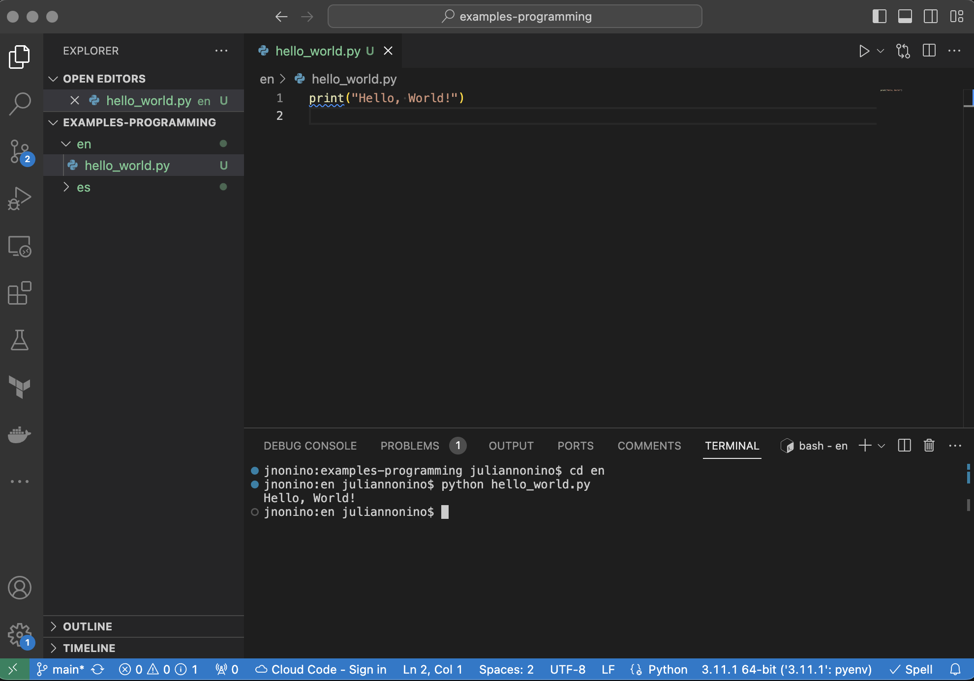
Hello, World!
This is arguably the most iconic program for beginners. It’s simple, but it introduces you to the process of writing and executing code.
print("Hello, World!")
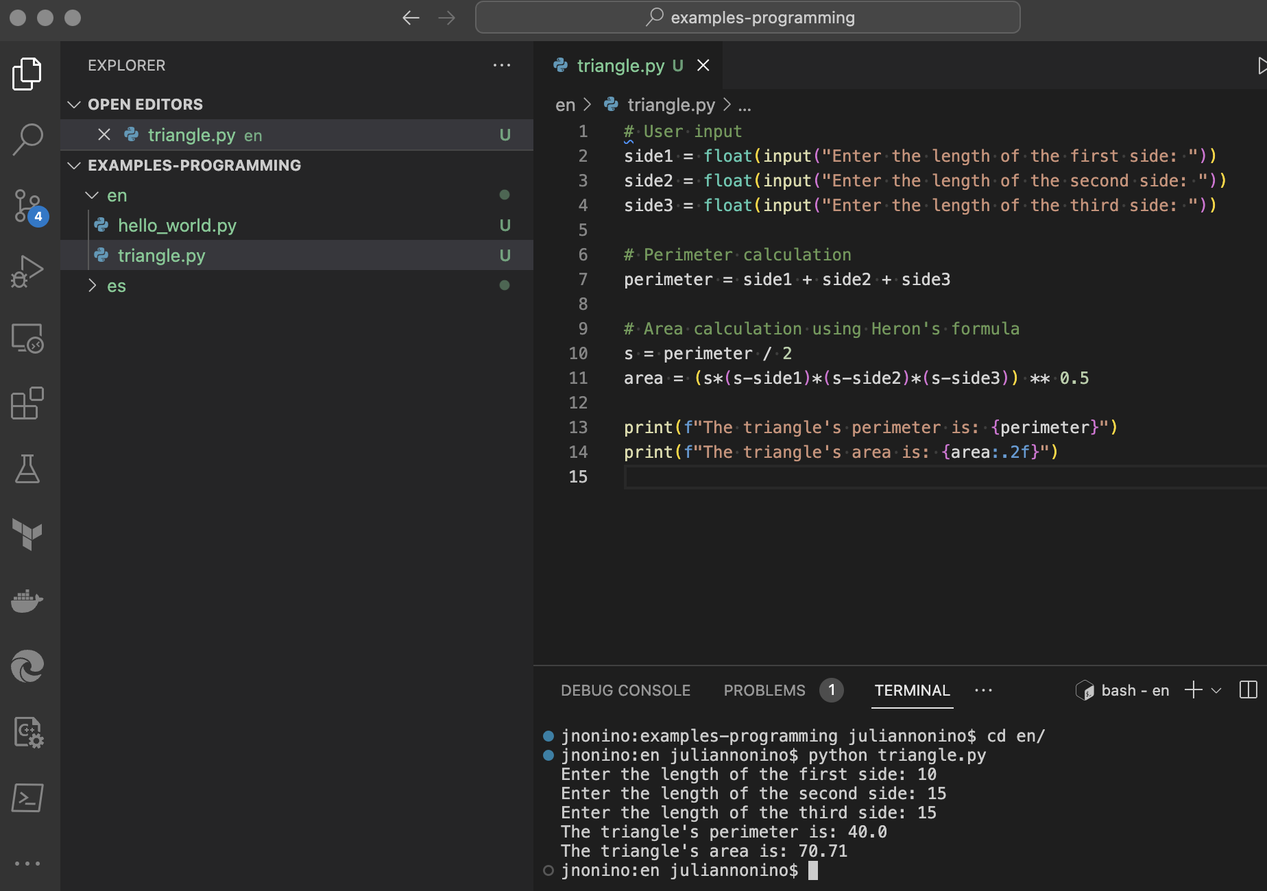
Triangle area and perimeter calculation
This program is a tad more intricate. It doesn’t just print out a message; it also performs mathematical calculations.
# User input
side1 = float(input("Enter the length of the first side: "))
side2 = float(input("Enter the length of the second side: "))
side3 = float(input("Enter the length of the third side: "))

# Perimeter calculation
perimeter = side1 + side2 + side3

# Area calculation using Heron's formula
s = perimeter / 2
area = (s*(s-side1)*(s-side2)*(s-side3)) ** 0.5

print(f"The triangle's perimeter is: {perimeter}")
print(f"The triangle's area is: {area:.2f}")
Conclusion
Setting up a programming environment might appear daunting at first, but with the right tools and resources, it becomes a manageable and rewarding task. We hope this article provided you with a solid foundation to kickstart your programming journey. Happy coding!
References
- Lutz, M. (2013). Learning Python. O’Reilly Media.
- Microsoft. (2020). Visual Studio Code Documentation. Microsoft Docs.
Cheers for making it this far! I hope this journey through the programming universe has been as fascinating for you as it was for me to write down.
We’re keen to hear your thoughts, so don’t be shy – drop your comments, suggestions, and those bright ideas you’re bound to have.
Also, to delve deeper than these lines, take a stroll through the practical examples we’ve cooked up for you. You’ll find all the code and projects in our GitHub repository learn-software-engineering/examples.
Thanks for being part of this learning community. Keep coding and exploring new territories in this captivating world of software!
2 - Starting Concepts
2.1 - Variables and Data Types
Variables
A variable is a container to store data in the computer’s memory. We can think of it as a box with a label. The label is the variable name and inside the box its value is stored.
To declare a variable in Python we just write the name and assign a value:
age = 28
price = 19.95
student = True
Variable names must start with letters or underscore, and can only contain letters, numbers and underscores. It is recommended to use meaningful names that represent the purpose of the variable.
In Python variables do not need to be declared with a particular type. The type is inferred automatically when assigning the value:
age = 28 # age is integer type
price = 19.95 # price is float type
single = True # single is boolean type
Once assigned, a variable can change its value at any time:
age = 30 # We change age to 30
Scope and lifetime
The scope of a variable refers to the parts of the code where it is available. Variables declared outside functions are global and available throughout the file. Variables inside a function are local and only visible within it.
The lifetime is the period during which the variable exists in memory. Local variables exist while the function executes, then they are destroyed. Global variables exist while the program is running.
Assignment
Assignment with the = operator allows changing or initializing a variable’s value:
number = 10
number = 20 # Now number is 20
There are also compound assignment operators like += and -= that combine an operation with assignment:
number += 5 # Adds 5 to number (number = number + 5)
number -= 2 # Subtracts 2 from number
Data types
Data types define what kind of value a variable can store. Python has several built-in types, including:
Numerical: To store integer, float, and complex numeric values:
integer = 10
float = 10.5
complex = 3 + 4j
Strings: To store text:
text = "Hello World"
Boolean: For True or False logical values:
true_variable = True
false_variable = False
Collections: To store multiple values like lists, tuples and dictionaries:
Lists: Mutable sequences of values:
list = [1, 2, 3]Tuples: Immutable sequences of values:
tuple = (1, 2, 3)Dictionaries: Key-value pair structures:
dictionary = {"name":"John", "age": 20}
It is important to choose the data type that best represents the information we want to store.
Operators
Operators allow us to perform operations with values and variables in Python. Some common operators are:
Arithmetic:
+, -, *, /, %, //, **Comparison:
==, !=, >, <, >=, <=Logical:
and, or, notAssignment:
=, +=, -=, *=, /=
Let’s see concrete examples of expressions using these operators in Python:
# Arithmetic
5 + 4 # Addition, result 9
10 - 3 # Subtraction, result 7
4 * 5 # Multiplication, result 20

# Comparison
5 > 4 # Greater than, result True
7 < 10 # Less than, result True

# Logical
True and False # Result False
True or False # Result True
not True # Result False

# Assignment
number = 10
number += 5 # Adds 5 to number, equivalent to number = number + 5
Each type of operator works with specific data types. We must use them consistently according to our variable data types.
Type conversions
Sometimes we need to convert one data type to another to perform certain operations. In Python we can convert explicitly or implicitly:
Explicit: Using functions like int(), float(), str():
float = 13.5
integer = int(float) # converts 13.5 to 13

text = "100"
number = int(text) # converts "100" to 100
Implicit: Python automatically converts in some cases:
integer = 100
float = 3.5
result = integer + float # result is 103.5, integer converted to float
Some conversions can generate data loss or errors:
float = 13.5
integer = int(float)

print(integer) # 13, decimals are lost
To prevent this we must explicitly choose conversions that make sense for our data.
Conclusion
In this article we reviewed key concepts like variables, operators, data types and conversions in Python. Applying these concepts well will allow you to efficiently manipulate data in your programs. I recommend practising with your own examples to gain experience using these features. Good luck in your Python learning!
Cheers for making it this far! I hope this journey through the programming universe has been as fascinating for you as it was for me to write down.
We’re keen to hear your thoughts, so don’t be shy – drop your comments, suggestions, and those bright ideas you’re bound to have.
Also, to delve deeper than these lines, take a stroll through the practical examples we’ve cooked up for you. You’ll find all the code and projects in our GitHub repository learn-software-engineering/examples.
Thanks for being part of this learning community. Keep coding and exploring new territories in this captivating world of software!
2.2 - Input and output operations
Screen output
Python also provides functions to send program output to “standard output”, usually the screen or terminal.
The print() function displays the value passed as a parameter:
name = "Eric"
print(name) # displays "Eric"
We can print multiple values separated by commas:
print("Hello", name, "!") # displays "Hello Eric!"
We can also use literal values without assigning to variables:
print("2 + 3 =", 2 + 3) # displays "2 + 3 = 5"
Output formatting
Python provides various ways to format output:
f-Strings: Allow inserting variables into a string:
name = "Eric"
print(f"Hello {name}") # displays "Hello Eric"
%s: Inserts string text into a format string:
name = "Eric"
print("Hello %s" % name) # displays "Hello Eric"
%d: Inserts integer numbers:
value = 15
print("The value is %d" % value) # displays "The value is 15"
.format(): Inserts values into a format string:
name = "Eric"
print("Hello {}. Welcome".format(name))
# displays "Hello Eric. Welcome"
These formatting options allow us to interpolate variables and values into text strings to generate custom outputs. We can combine multiple values and formats in a single output string.
Keyboard input
Python provides built-in functions to read data entered by the user at runtime. This is known as “standard input”.
The input() function allows reading a value entered by the user and assigning it to a variable. For example:
name = input("Enter your name: ")
This displays the message “Enter your name: " and waits for the user to enter text and press Enter. That value is assigned to the name variable.
The input() function always returns a string. If we want to ask for a number or other data type, we must convert it using int(), float(), etc:
age = int(input("Enter your age: "))
pi = float(input("Enter the value of pi: "))
Reading multiple values
We can ask for and read multiple values on the same line separating them with commas:
name, age = input("Enter name and age: ").split()
The split() method divides the input into parts and returns a list of strings. We then assign the list elements to separate variables.
We can also read multiple lines of input with a loop:
names = [] # empty list

for x in range(3):
   name = input("Enter a name: ")
   names.append(name)
This code reads 3 names entered by the user and adds them to a list.
Output to a file
In addition to printing to the screen, we can write output to a file using the open() function:
file = open("data.txt", "w")
This opens data.txt for writing (“w”) and returns a file object.
Then we use file.write() to write to that file:
file.write("Hello World!")
file.write("This text goes to the file")
We must close the file with file.close() when finished:
file.close()
We can also use with to open and automatically close:
with open("data.txt", "w") as file:
   file.write("Hello World!")
   # no need to close, it's automatic
Reading files
To read a file we use open() in “r” mode and iterate over the file object:
with open("data.txt", "r") as file:
   for line in file:
      print(line) # prints each line of the file
This prints each line, including newlines.
We can read all lines to a list with readlines():
lines = file.readlines()
print(lines)
To read the full content to a string we use read():
text = file.read()
print(text)
We can also read a specific number of bytes or characters with read(n).
File handling operations
There are several built-in functions to handle files in Python:
open()- Opens a file and returns a file objectclose()- Closes the filewrite()- Writes data to the fileread()- Reads data from the filereadline()- Reads a line from the filetruncate()- Empties the fileseek()- Changes the reading/writing positionrename()- Renames the fileremove()- Deletes the file
These allow us to perform advanced operations to read, write and maintain files.
Conclusion
In this article we explained Python input and output operations in detail, including reading from standard input and writing to standard output or files. Properly handling input and output is essential for many Python applications. I recommend practising with your own examples to master these functions.
References
- Downey, A. B. (2015). Think Python: How to think like a computer scientist. Needham, Massachusetts: Green Tea Press.
- McKinney, W. (2018). Python for data analysis: Data wrangling with Pandas, NumPy, and IPython. O’Reilly Media.
- Matthes, E. (2015). Python crash course: A hands-on, project-based introduction to programming. No Starch Press.
- Lutz, M. (2013). Learning Python: Powerful Object-Oriented Programming. O’Reilly Media, Incorporated.
Cheers for making it this far! I hope this journey through the programming universe has been as fascinating for you as it was for me to write down.
We’re keen to hear your thoughts, so don’t be shy – drop your comments, suggestions, and those bright ideas you’re bound to have.
Also, to delve deeper than these lines, take a stroll through the practical examples we’ve cooked up for you. You’ll find all the code and projects in our GitHub repository learn-software-engineering/examples.
Thanks for being part of this learning community. Keep coding and exploring new territories in this captivating world of software!
2.3 - Flow Control
Conditions: making decisions in code
Life is full of decisions: “If it rains, I’ll take an umbrella. Otherwise, I’ll wear sunglasses.” These decisions are also present in the world of programming. Conditions are like questions the computer asks itself. They allow us to make decisions and execute specific code based on a condition. They can be as simple as “Is it raining?” or as complex as “Is it the weekend and do I have less than $100 in my bank account?”.
if
The if structure allows us to evaluate conditions and make decisions based on the result of that evaluation.
age = 15

if age >= 18:
    print("You are an adult")
The code above allows executing a portion of code if a person’s age is greater than or equal to 18 years.
if-else
When you want to execute alternative code if the condition is false, you use the if-else structure.
age = 21
if age >= 18:
    print("You are an adult")
else:
    print("You are a minor")
In this case, it determines if the person is an adult or a minor, and the message displayed is different.
if-elif-else
When conditions are multiple and two paths are not enough, the if-elif-else structure is used to evaluate them in a chained way.
age = 5
if age <= 13:
    print("You are a child")
elif age > 13 and age < 18:
    print("You are a teenager")
else:
    print("You are an adult")
In the code above, there are three clear paths: one for when age is less than or equal to 13, one for when age is between 13 and 18, and another for when age is greater than or equal to 18.
Another way to solve this problem is through the switch-case structure, which, although Python does not natively incorporate, other languages like Java or C++ do, and it is an important tool to be familiar with. This structure allows programmers to handle multiple conditions in a more organized way than a series of if-elif-else.
In Java, for example:
int day = 3;
switch(day) {
  case 1:
    System.out.println("Monday");
    break;
  case 2:
    System.out.println("Tuesday");
    break;
  case 3:
    System.out.println("Wednesday");
    break;
  // ... and so on
  default:
    System.out.println("Invalid day");
}
In the previous example, depending on the value of day, the corresponding day will be printed.
Loops: repeating actions
Sometimes in programming we need to repeat an action several times. Instead of writing the same code many times, we can use loops. These allow repeating the execution of a block of code while a condition is met.
while
The while loop is useful when we want to repeat an action based on a condition.
# Prints 1 to 5
i = 1
while i <= 5:
    print(i)
    i = i + 1
do-while
Similar to while but guarantees at least one execution since the code block is executed first and then the condition is evaluated. Python does not implement this structure, but other languages like Java and C++ do.
int i = 1;

do {
  System.out.println(i);
  i++;
} while(i <= 5);
int number = 0;
do {
  std::cout << "Hello, world!" << std::endl;
  number++;
} while (number < 5);
for
The for loop is useful when we know how many times we want to repeat an action.
for i in range(5):
    print("Hello, world!")
The code above will print “Hello, world!” five times.
We can also iterate over the elements of a list or iterable object:
names = ["Maria", "Florencia", "Julian"]
for name in names:
    print(f"Hello {name}")

# Prints
# Hello Maria
# Hello Florencia
# Hello Julian
The break and continue statements
We can use break to terminate the loop and continue to skip to the next iteration.
break is used to completely terminate the loop when a condition is met, in the following example, when i reaches 5.
# break example
i = 0
while i < 10:
  print(i)
  if i == 5:
    break
  i += 1

# Prints:
# 0
# 1
# 2
# 3
# 4
# 5
continue is used to skip an iteration of the loop and continue with the next one when a condition is met. Here we use it to skip even numbers.
# continue example
i = 0
while i < 10:
  i += 1
  if i % 2 == 0:
    continue
  print(i)

# Prints:
# 1
# 3
# 5
# 7
# 9
Nesting: combining structures
Control flow structures can be nested within each other. For example, we can have loops within loops or conditions within loops.
for i in range(5):
  for j in range(10):
    if (i % 2 == 0 and j % 3 == 0):
      print(f"i = {i}, j = {j}")
This code will print combinations of i and j only when i is divisible by 2 and j is divisible by 3, demonstrating how loops are nested and executed.
Common usage patterns
There are specific patterns to solve common needs with control flow.
Search
Search for a value in a collection:
fruits = ["apple", "orange"]

searching = "orange"
found = False

for fruit in fruits:
    if fruit == searching:
        found = True
        break

if found:
    print("Fruit found!")
Accumulation
Accumulate incremental values in a loop:
total = 0

for i in range(10):
    total += i

print(total) # Sum from 0..9 = 45
Flowcharts: the visual route to understanding code
Programmers, whether beginners or experts, often find themselves facing challenges that require detailed planning before diving into code. This is where flowcharts come into play as an essential tool. These charts are graphical representations of the processes and logic behind a program or system. In this article, we will unravel the world of flowcharts, from basic concepts to advanced techniques, and how they can benefit programmers of all levels.
A flowchart is a graphical representation of a process. It uses specific symbols to represent different types of instructions or actions. Its main purpose is to simplify understanding of a process by showing step by step how information or decisions flow. These charts:
- Facilitate understanding of complex processes.
- Aid in the design and planning phase of a program.
- Serve as documentation and reference for future developments.
Flowcharts are a powerful tool that not only benefits beginners but also experienced programmers. They provide a clear and structured view of a process or program, facilitating planning, design, and communication between team members.
Basic elements
Flowcharts consist of several symbols, each with a specific meaning:
- Oval: Represents the start or end of a process.
- Rectangle: Denotes an operation or instruction.
- Diamond: Indicates a decision based on a condition.
- Arrows: Show the direction of flow.
graph TD;
    start((Start))
    process[Process]
    decision{Decision?}
    final((End))

    start --> process;
    process --> decision;
    decision --> |Yes| process
    decision --> |No| final
Examples
Let’s design a flowchart for a program that asks for a number and tells us if it’s even or odd.
graph TB
    start((Start))
    input[Input number]
    decision{Even?}
    isEven[Is even]
    isOdd[Is odd]
    final((End))

    start --> input
    input --> decision
    decision --> |Yes| isEven
    decision --> |No| isOdd
    isEven --> final
    isOdd --> final
As programs become more complex, you may need to incorporate loops, multiple conditions, and other advanced elements into your flowchart. For example, here we diagram a program that sums numbers from 1 to a number entered by the user.
graph TD
    start((Start))
    input[Input number]
    setVariables[Set sum=0 and counter=1]
    loop_condition{counter <= N?}
    loop_code[Add value and increment counter]
    result[Show sum]
    final((End))

    start --> input
    input --> setVariables
    setVariables --> loop_condition
    loop_condition --> |Yes| loop_code
    loop_code --> loop_condition
    loop_condition --> |No| result
    result --> final
Conclusion
Control flow is the heart of programming. Without it, programs would be linear sequences of actions without the ability to make decisions or repeat tasks. By mastering these structures not only do you improve your ability to write code, but also your ability to think logically and solve complex problems.
References
- Lutz, M. (2013). Learning Python: Powerful Object-Oriented Programming. O’Reilly Media, Incorporated.
- Deitel, P., & Deitel, H. (2012). Java: How to program. Upper Saddle River, NJ: Prentice Hall.
- Matthes, E. (2015). Python crash course: A hands-on, project-based introduction to programming. San Francisco, CA: No Starch Press.
Cheers for making it this far! I hope this journey through the programming universe has been as fascinating for you as it was for me to write down.
We’re keen to hear your thoughts, so don’t be shy – drop your comments, suggestions, and those bright ideas you’re bound to have.
Also, to delve deeper than these lines, take a stroll through the practical examples we’ve cooked up for you. You’ll find all the code and projects in our GitHub repository learn-software-engineering/examples.
Thanks for being part of this learning community. Keep coding and exploring new territories in this captivating world of software!
2.4 - Functions
What are functions?
A function, in simple terms, is a block of code that executes only when called. You can think of it as a small program within your main program, designed to perform a specific task. A function can also be seen as a black box: we pass an input (parameters), some internal processing occurs, and it produces an output (return value).
Functions allow us to segment our code into logical parts where each part performs a single action. This provides several benefits:
- Reusability: Once defined, we can execute (call) that code from anywhere in our program as many times as needed.
- Organization: It allows dividing a large program into smaller, more manageable parts.
- Encapsulation: Functions reduce complexity by hiding internal implementation details.
- Maintainability: If we need to make changes, we only have to modify the code in one place (the function) instead of tracking down all instances of that code.
Procedures vs. Functions
It is vital to distinguish between these two concepts. While a function always returns a value, a procedure performs a task but does not return anything. In some languages, this difference is clearer than in others. Python, for example, has functions that can optionally return values.
Anatomy of a function
In Python, a function is declared using the def keyword, followed by the function name and parentheses. The code inside the function is called the body of the function and contains the set of instructions to execute to perform its task.
def my_function():
    print("Hello from my function!")
To call or invoke a function, we simply use its name followed by parentheses:
my_function() # Output: Hello from my function!
Parameters and arguments
Functions become even more powerful when we pass information to them, known as parameters. These act as “variables” inside the function, allowing the function to work with different data each time it is called.
While parameters are variables defined in the function definition, arguments are the actual values passed when calling the function.
def greet(name):
    print(f"Hello {name}!")

greet("Maria")
# Output:
#   Hello Maria!
Python allows default parameters, which have a predetermined value, making passing those arguments optional when calling the function. It also allows named parameters which enable passing arguments in any order by specifying their name.
def greet(name="Maria", repetitions=3):
    repetition = 1
    while repetition <= repetitions:
        print(f"Hello {name}!")
        repetition += 1

greet()
# Output:
#   Hello Maria!
#   Hello Maria!
#   Hello Maria!

greet("Florencia", 4)
# Output:
#   Hello Florencia!
#   Hello Florencia!
#   Hello Florencia!
#   Hello Florencia!

greet(repetitions=2, name="Julian")
# Output
#   Hello Julian!
#   Hello Julian!
Returning values
Functions can return a result or return value using the return keyword.
def circle_area(radius):
    return 3.14 * (radius ** 2)

result = circle_area(10)
print(result) # Output: 314
The return value is passed back to where the function was called and can be assigned to a variable for later use.
Functions can also perform some task without explicitly returning anything. In Python this is known as returning None.
Local and global variables
Local variables are defined inside a function and only exist in that scope, while global variables are defined outside and can be accessed from anywhere in the code. It is crucial to understand their scope (where a variable is accessible) and lifetime (how long a variable lives).
x = 10 # x is global

def add():
    y = 5 # y is local
    return x + y

add() # Output: 15
print(y) # Error, y does not exist outside the function
We can read global variables from a function, but if we need to modify it we must declare it global.
x = 10

def add():
    global x
    x = x + 5

add()
print(x) # 15
Best Practices
When creating functions we should follow certain principles and patterns:
- The name of a function should clearly indicate its purpose.
- Make functions small, simple, and focused on one task. A function should do one thing and do it well.
- Use descriptive names for functions and parameters.
- Avoid side effects and modifying global variables.
- Properly document the purpose and usage of each function.
- Limit the number of parameters, ideally 0 to 3 parameters.
Following these best practices will help us create reusable, encapsulated, and maintainable functions.
Conclusion
Functions are core components in programming, allowing us to organize, reuse, and encapsulate code. By defining functions that perform a single task we keep our programs simplified, easy to understand, and modify. By understanding and mastering this concept, you not only improve the quality of your code but also your efficiency as a developer.
References
- McConnell, S. (2004). Code Complete. Microsoft Press.
- Joyanes Aguilar, L. (2008). Fundamentos de programación: algoritmos, estructura de datos y objetos. McGraw-Hill.
- Kindler, E., & Krivy, I. (2011). Object-Oriented Simulation of systems with Java: A working introduction. BoD–Books on Demand.
- Python Software Foundation. (2022). Python Official Documentation.
Cheers for making it this far! I hope this journey through the programming universe has been as fascinating for you as it was for me to write down.
We’re keen to hear your thoughts, so don’t be shy – drop your comments, suggestions, and those bright ideas you’re bound to have.
Also, to delve deeper than these lines, take a stroll through the practical examples we’ve cooked up for you. You’ll find all the code and projects in our GitHub repository learn-software-engineering/examples.
Thanks for being part of this learning community. Keep coding and exploring new territories in this captivating world of software!
2.5 - Recursive Functions
Recursion: the art of calling yourself
Imagine a box of mirrors where each mirror reflects what it sees in the next, creating an infinite series of reflections. Recursion in programming is something similar. It is a technique where a function calls itself directly or indirectly. This creates a cycle where the function solves a problem by dividing it into smaller instances of the same problem, until reaching a simple base case that can be solved directly.
For example, let’s imagine a function that prints a countdown:
def countdown(number):

    if number > 0:
        print(number)
        countdown(number - 1)
    else:
        print("Blastoff!")

countdown(5)
This function calls itself recursively decrementing the number each time until reaching 0, and then prints the blastoff message.
Recursion is a declarative approach that focuses on dividing a problem into recursive cases without needing to explicitly control the loop using iterators or counters like in imperative programming.
The structure of a recursive function
The power of recursion lies in its simplicity. However, it is essential to understand its structure to avoid common pitfalls. A typical recursive function has two main parts:
- Base case: The simplest case with a known solution that doesn’t require recursion. It is the stopping condition that halts the recursion. Without a base case, we would fall into infinite recursion which eventually overflows the call stack.
- Recursive case: This is where the magical recursive call occurs. At this point, the function calls itself with a modified argument, usually a reduced version of the original problem.
Classic recursion examples
Factorial
The factorial of a positive integer \(n\) is the product of all positive integers less than or equal to \(n\). For example:
- \(5! = 5 * 4 * 3 * 2 * 1 = 120\)
- \(4! = 4 * 3 * 2 * 1 = 24\)
- \(3! = 3 * 2 * 1 = 6\)
Here is the Python code for calculating factorial using recursion:
def factorial(n):
    if n == 1:
        return 1       # Base case
    return n * factorial(n-1) # Recursive case
- Base case: The base case is the simplest, smallest instance of the problem that can be answered directly. For factorial, when \(n = 1\), the result is \(1\).
- Recursive case: If \(n\) is greater than \(1\), the function calls itself with \(n-1\), and multiplies the result by \(n\).
Let’s say you want to calculate the factorial of \(5\), so you call factorial(5).
Here is what happens:
- Step 1: Since \(n = 5\) is not \(1\), the function calls
factorial(4), then multiplies the result by \(5\). - Step 2: Now, inside
factorial(4), \(n = 4\), so the function callsfactorial(3), then multiplies the result by \(4\). - Step 3: Inside
factorial(3), \(n = 3\), so it callsfactorial(2), then multiplies the result by \(3\). - Step 4: Inside
factorial(2), \(n = 2\), so it callsfactorial(1), then multiplies the result by \(2\). - Step 5: Finally,
factorial(1)reaches the base case, where \(n = 1\), so it returns \(1\).
Now the results unwind:
factorial(2)returns \(2 * 1 = 2\)factorial(3)returns \(3 * 2 = 6\)factorial(4)returns \(4 * 6 = 24\)factorial(5)returns \(5 * 24 = 120\)
The final result is \(120\), which is the value of \(5!\).
Here is a visual representation of the call stack:
factorial(5)
  -> factorial(4)
    -> factorial(3)
      -> factorial(2)
        -> factorial(1)
          return 1
        return 2
      return 6
    return 24
  return 120
Fibonacci sequence
The Fibonacci sequence is a series of numbers where each number is the sum of the previous two. It starts with \(0\) and \(1\), and each subsequent number is the sum of the two numbers before it. The beginning of the sequence is: \(0, 1, 1, 2, 3, 5, 8, 13, 21, 34, …\)
Here is the Python code for calculating the \(n^th\) Fibonacci number using tail recursion:
def fibonacci(n, a=0, b=1):
    if n == 0:
        return a
    return fibonacci(n-1, b, a+b)
The function takes three parameters:
- \(n\): The position of the desired number in the sequence.
- \(a\) and \(b\): Two numbers that aid in the sequence calculation.
Here is a breakdown of how the function works:
- Base case: If \(n\) is \(0\), the function returns \(a\). This is the value of the \(n^th\) number in the sequence.
- Recursive case: If \(n\) is not \(0\), the function calls itself with \(n-1\), \(b\), and \(a+b\). These parameters change the position in the sequence and prepare the next numbers for summation.
Suppose we want to find the \(5^th\) number in the Fibonacci sequence by calling fibonacci(5).
Here is what happens:
- Step 1: Since \(n = 5\), it calls
fibonacci(4, 1, 1)(because \(a = 0\), \(b = 1\), \(a + b = 1\)). - Step 2: Since \(n = 4\), it calls
fibonacci(3, 1, 2)(because \(a = 1\), \(b = 1\), \(a + b = 2\)). - Step 3: Since \(n = 3\), it calls
fibonacci(2, 2, 3)(because \(a = 1\), \(b = 2\), \(a + b = 3\)). - Step 4: Since \(n = 2\), it calls
fibonacci(1, 3, 5)(because \(a = 2\), \(b = 3\), \(a + b = 5\)). - Step 5: Since \(n = 1\), it calls
fibonacci(0, 5, 8)(because \(a = 3\), \(b = 5\), \(a + b = 8\)). - Step 6: Since \(n = 0\), it returns \(a\), which is \(5\).
The result is \(5\), which is the \(5^th\) number in the Fibonacci sequence.
Here is a visual representation of the call stack:
fibonacci(5, 0, 1)
  -> fibonacci(4, 1, 1)
    -> fibonacci(3, 1, 2)
      -> fibonacci(2, 2, 3)
        -> fibonacci(1, 3, 5)
          -> fibonacci(0, 5, 8)
            return 5
Advantages and Disadvantages
Recursion has certain advantages:
- It can result in simple, elegant solutions for problems that easily break down into subproblems.
- It eliminates the need for explicit loop control.
- It mirrors the mathematical structure of a recursive definition.
The disadvantages include:
- It can be less efficient (high memory consumption) than iteration due to repeated function calls and stack frame creation.
- Too much recursion can overflow the call stack and cause crashes.
- It can be harder to debug and analyze than iteration.
Therefore, recursion is a powerful tool that should be used judiciously in appropriate cases.
Recursion vs Iteration
Recursion and iteration (using loops) are parallel tools and we can use either one to solve many problems. Both techniques have the potential to solve the same problems, but their implementation and efficiency may vary. Let’s take the factorial example:
Iterative
def factorial_iterative(n):
    result = 1
    for i in range(1, n+1):
        result *= i
    return result
Recursive
def factorial_recursive(n):
    if n == 1:
        return 1
    return n * factorial(n-1)
The iterative version is more efficient in terms of space, but the recursive is cleaner and easier to understand. The choice between recursion and iteration often depends on the specific problem, memory constraints, and programmer preferences.
Conclusion
Recursion is a key technique that allows writing elegant, natural, and efficient algorithms when properly leveraged. Understanding how to break down a problem into recursive cases is essential to master this skill. Recursion provides a unique declarative alternative to solve complex problems without managing explicit loops. However, it is crucial to always remember to define an adequate base case and be aware of recursion limitations in terms of efficiency and memory usage. Knowing how to combine recursion and iteration gives flexibility when creating optimal solutions.
As always, the key lies in finding the right balance and using the right tool for the right job.
References
- Cormen, T.H., Leiserson, C.E., Rivest, R.L., & Stein, C. (2009). Introduction to Algorithms. MIT Press.
- Kindler, E., & Krivy, I. (2011). Object-Oriented Simulation of systems with Java: A working introduction. BoD–Books on Demand.
- Lutz, M. (2013). Learning Python: Powerful Object-Oriented Programming. O’Reilly Media, Incorporated.
Cheers for making it this far! I hope this journey through the programming universe has been as fascinating for you as it was for me to write down.
We’re keen to hear your thoughts, so don’t be shy – drop your comments, suggestions, and those bright ideas you’re bound to have.
Also, to delve deeper than these lines, take a stroll through the practical examples we’ve cooked up for you. You’ll find all the code and projects in our GitHub repository learn-software-engineering/examples.
Thanks for being part of this learning community. Keep coding and exploring new territories in this captivating world of software!
3 - Object-Oriented Programming
Object-Oriented Programming (OOP) is a programming paradigm that has become indispensable nowadays. This approach models real-world elements as “objects” that have properties and behaviours, which allows for more intuitive and maintainable programmes to be created. In this article we will look at the basic concepts of OOP and its advantages over other paradigms like procedural programming. Let’s get started!
This paradigm is based on two fundamental concepts:
- Objects: entities that combine state (data) and behaviour (operations) in a single unit. For example, a “car” object would have properties like colour, number of doors, maximum speed, etc. And behaviours like accelerate, brake, steer, etc.
- Classes: specifications that define the common structure and behaviour of a group of objects. The “car” class would serve as a template for creating car objects with the same characteristics.
As explained by programmer Alan Kay, one of the creators of OOP:
“The big idea is to design programmes in terms of conceptual objects and concepts from the real world. The interfaces with the real world should, therefore, be constructed in terms of these conceptual objects.”
That is, OOP conceptually models real-world elements to make programming more intuitive.
Programming paradigms
Before delving into OOP, it is worth understanding that there are different paradigms or approaches to tackle programming. The main ones are:
Procedural programming
Ordered sequence of instructions that the programme must follow step-by-step. The focus is on procedures and functions. For example, C is a language geared towards procedural programming.
Procedural programming is better for:
- Simple problems or sequential algorithms.
- Code that won’t need heavy reusing or expanding.
- Cases where performance and efficiency are critical.
Object-Oriented programming
Model based on objects that contain data and code in cohesive units. The focus is on classes and the interaction between objects. For example, Java and Python are object-oriented languages.
OOP allows modelling real-world elements more directly, better encapsulating data, and reusing code through inheritance between classes.
The main advantages of OOP over procedural programming are:
- Modularity: objects group related data and operations, encapsulating internal complexity. This allows working with independent modules.
- Information hiding: Objects can expose a simple interface and hide internal implementation details. This reduces coupling.
- Reusability: Classes enable code reuse. An abstract class can inherit to multiple subclasses.
- Extensibility: We can extend the behaviour of parent classes by creating new subclasses.
- Conceptual mapping: Objects represent real-world entities, which eases the translation of requirements into code.
However, OOP also has disadvantages. According to programmer Paul Graham:
“Object-oriented programming often makes things harder than they need to be.”
For example, for simple problems OOP can be excessive. And in large projects there is a risk of overusing inheritance and polymorphism, making the code difficult to follow.
Ultimately, OOP is more suitable when:
- The problem to be modelled has clear, structured entities.
- We want to reuse encapsulated code in modular classes.
- We work on systems that need to be easily extended and maintained.
More articles
3.1 - Classes and objects
Anatomy of a class
A class acts as a blueprint or mould to construct similar objects, defining their common characteristics and functionalities. It is similar to the blueprint used to construct houses in the same neighbourhood: they all share certain key attributes.
The typical components of a class are:
Attributes (properties): Variables that characterise the object. For example, for a Person class, attributes like name, age, ID, etc.
class Person:
  id = ""
  name = ""
  age = 0
Methods: Functions that define behaviours. For example, a Person can walk(), talk(), eat(), etc. They access the attributes to implement said functionality.
Constructor: Special __init__() method that executes when instantiating the class and allows initialising attributes.
Destructor: __del__() method that executes when deleting the instance, freeing up resources. Optional in some languages.
Creating objects
From the class we generate objects, which are specific instances with their own defined attributes. Let’s say the House class is the blueprint, and a specific house on a particular street is the object.
In code, we create an object by invoking the class as if it were a method:
# Person class
class Person:
  def __init__(self, n, a):
    self.name = n
    self.age = a

# Specific Person objects
john = Person("John", 30)
mary = Person("Mary", 35)
Each object shares the general structure and behaviour but can store different data.
Using properties and methods
We now have a Person class and a john object of type Person. How do we interact with the object?
- Properties: It is possible to access the value of an object attribute using the object reference (
john) and the attribute name.
john.name  # "John"
john.age   # 30
- Methods: Are invoked in the same way as accessing attributes but adding parentheses, and inside them, the arguments that are passed if it takes any.
# Person class
class Person:
  def __init__(self, n, a):
      self.name = n
      self.age = a

  def eat(self, food):
      print(f"Eating {food}")

# Specific Person object
john = Person("John", 30)
john.eat("pizza") # Prints "Eating pizza"
The john object now has its own state (properties) and behaviour (methods).
Self vs This
An important detail in methods is how they access the object’s attributes and other methods. Here another difference between languages comes into play:
- Self: In Python, attributes and methods are accessed within the class by prepending
self. This points to the instantiated object.
class Person:

  def __init__(self, name):
    self.name = name

  def greet(self):
    print(f"Hello! I'm {self.name}")

john = Person("John")
john.greet()
# Prints "Hello! I'm John"
- This: In Java or C#,
thisis used instead of self. It fulfils the same functionality of pointing to the object’s members.
public class Person {

  private String name;

  public Person(String name) {
    this.name = name;
  }

  public void greet() {
    System.out.println("Hello! I'm " + this.name);
  }
}

Person john = new Person("John");
john.greet();
// Prints "Hello! I'm John"
Conclusion
Classes and objects are the key concepts in OOP, allowing modelling real-world entities and generating modular, generic components of our system to construct more robust and easy to understand programmes.
Cheers for making it this far! I hope this journey through the programming universe has been as fascinating for you as it was for me to write down.
We’re keen to hear your thoughts, so don’t be shy – drop your comments, suggestions, and those bright ideas you’re bound to have.
Also, to delve deeper than these lines, take a stroll through the practical examples we’ve cooked up for you. You’ll find all the code and projects in our GitHub repository learn-software-engineering/examples.
Thanks for being part of this learning community. Keep coding and exploring new territories in this captivating world of software!
3.2 - Class relations
In Object-Oriented Programming, classes don’t exist in isolation. They interact and relate to each other in various ways to model complex systems and relationships. Understanding these relationships is crucial for designing effective and maintainable object-oriented systems.
The main types of class relationships we’ll explore in depth are:
- Association (“uses-a”)
- Aggregation (weak “has-a” relationship)
- Composition (strong “has-a” relationship)
- Inheritance (“is-a” relationship)
- Realisation (Implementation)
- Dependency
Each of these relationships represents a different way that classes can be connected and interact with each other. They vary in terms of the strength of the coupling between classes, the lifecycle dependencies, and the nature of the relationship.
Before we dive into each type of relationship, let’s visualise them using a UML class diagram:
classDiagram
    class ClassA
    class ClassB
    class ClassC
    class ClassD
    class ClassE
    class ClassF
    class InterfaceG

    ClassA --> ClassB : Association
    ClassC o-- ClassD : Aggregation
    ClassE *-- ClassF : Composition
    ClassB --|> ClassA : Inheritance
    ClassE ..|> InterfaceG : Realisation
    ClassA ..> ClassF : Dependency
This diagram provides a high-level overview of the different types of class relationships. In the following sections, we’ll explore each of these relationships in detail, providing explanations, examples, and more specific UML diagrams.
3.2.1 - Association
Key characteristics of association:
- It represents a loose coupling between classes.
- The associated classes can exist independently of each other.
- The lifetime of one class is not tied to the lifetime of the other.
- It can be unidirectional or bidirectional.
There are two main types of association:
- Unidirectional Association
- Bidirectional Association
Let’s explore each of these in more detail.
Unidirectional association
In a unidirectional association, one class knows about and can interact with another class, but not vice versa. This is a one-way relationship.
Here’s an example in Python:
class Customer:
    def __init__(self, name):
        self.name = name

class Order:
    def __init__(self, order_number, customer):
        self.order_number = order_number
        self.customer = customer  # This creates an association

    def display_info(self):
        return f"Order {self.order_number} placed by {self.customer.name}"

# Creating instances
customer = Customer("John Doe")
order = Order("12345", customer)

print(order.display_info())  # Output: Order 12345 placed by John Doe
In this example, the Order class has a unidirectional association with the Customer class. An Order knows about its associated Customer, but a Customer doesn’t know about its Orders.
Here’s a UML diagram representing this relationship:
classDiagram
    class Customer {
        +name: string
    }
    class Order {
        +order_number: string
        +customer: Customer
        +display_info()
    }
    Order --> Customer : places
The arrow in the diagram points from Order to Customer, indicating that Order knows about Customer, but not the other way around.
Bidirectional association
In a bidirectional association, both classes are aware of each other and can interact with each other. This is a two-way relationship.
Here’s an example in Python:
class Student:
    def __init__(self, name):
        self.name = name
        self.courses = []

    def enroll(self, course):
        self.courses.append(course)
        course.add_student(self)

    def display_courses(self):
        return f"{self.name} is enrolled in: {', '.join(course.name for course in self.courses)}"

class Course:
    def __init__(self, name):
        self.name = name
        self.students = []

    def add_student(self, student):
        self.students.append(student)

    def display_students(self):
        return f"{self.name} has students: {', '.join(student.name for student in self.students)}"

# Creating instances
student1 = Student("Alice")
student2 = Student("Bob")
math_course = Course("Mathematics")
physics_course = Course("Physics")

# Enrolling students in courses
student1.enroll(math_course)
student1.enroll(physics_course)
student2.enroll(math_course)

print(student1.display_courses())
print(math_course.display_students())
In this example, there’s a bidirectional association between Student and Course. A Student knows about their Courses, and a Course knows about its Students.
Here’s a UML diagram representing this relationship:
classDiagram
    class Student {
        +name: string
        +courses: list
        +enroll(course)
        +display_courses()
    }
    class Course {
        +name: string
        +students: list
        +add_student(student)
        +display_students()
    }
    Student "0..*" <--> "0..*" Course : enrolls in >
The double-headed arrow in the diagram indicates that both Student and Course are aware of each other. The “0..*” notation indicates that a Student can be enrolled in zero or more Courses, and a Course can have zero or more Students.
Association is a flexible relationship that can represent many real-world connections between objects. It’s important to choose between unidirectional and bidirectional associations carefully, as bidirectional associations can introduce more complexity and potential for errors if not managed properly.
References
- Gamma, E., Helm, R., Johnson, R., & Vlissides, J. (1994). Design Patterns: Elements of Reusable Object-Oriented Software. Addison-Wesley.
- Martin, R. C. (2017). Clean Architecture: A Craftsman’s Guide to Software Structure and Design. Prentice Hall.
- Fowler, M. (2002). Patterns of Enterprise Application Architecture. Addison-Wesley.
- Bloch, J. (2018). Effective Java (3rd ed.). Addison-Wesley.
- Phillips, D. (2018). Python 3 Object-Oriented Programming (3rd ed.). Packt Publishing.
- Lott, S. F. (2020). Object-Oriented Python: Master OOP by Building Games and GUIs. No Starch Press.
- Booch, G., Rumbaugh, J., & Jacobson, I. (2005). The Unified Modeling Language User Guide (2nd ed.). Addison-Wesley.
Cheers for making it this far! I hope this journey through the programming universe has been as fascinating for you as it was for me to write down.
We’re keen to hear your thoughts, so don’t be shy – drop your comments, suggestions, and those bright ideas you’re bound to have.
Also, to delve deeper than these lines, take a stroll through the practical examples we’ve cooked up for you. You’ll find all the code and projects in our GitHub repository learn-software-engineering/examples.
Thanks for being part of this learning community. Keep coding and exploring new territories in this captivating world of software!
3.2.2 - Aggregation
Key characteristics of aggregation:
- It’s a stronger relationship than a simple association, but weaker than composition.
- The “part” object can exist independently of the “whole” object.
- Multiple “whole” objects can share the same “part” object.
- If the “whole” object is destroyed, the “part” object continues to exist.
Let’s look at an example to illustrate aggregation:
class Department:
    def __init__(self, name):
        self.name = name
        self.employees = []

    def add_employee(self, employee):
        self.employees.append(employee)

    def remove_employee(self, employee):
        self.employees.remove(employee)

    def list_employees(self):
        return f"Department {self.name} has employees: {', '.join(emp.name for emp in self.employees)}"

class Employee:
    def __init__(self, name, id):
        self.name = name
        self.id = id

    def __str__(self):
        return f"Employee(name={self.name}, id={self.id})"

# Creating instances
hr_dept = Department("Human Resources")
it_dept = Department("Information Technology")

emp1 = Employee("Alice", "E001")
emp2 = Employee("Bob", "E002")
emp3 = Employee("Charlie", "E003")

# Adding employees to departments
hr_dept.add_employee(emp1)
hr_dept.add_employee(emp2)
it_dept.add_employee(emp2)  # Note: Bob works in both HR and IT
it_dept.add_employee(emp3)

print(hr_dept.list_employees())
print(it_dept.list_employees())

# If we remove the HR department, the employees still exist
del hr_dept
print(emp1)  # Employee still exists
In this example, we have an aggregation relationship between Department and Employee. A Department has Employees, but Employees can exist independently of any particular Department. Also, an Employee can belong to multiple Departments (as we see with Bob).
Here’s a UML diagram representing this aggregation relationship:
classDiagram
    class Department {
        +name: string
        +employees: list
        +add_employee(employee)
        +remove_employee(employee)
        +list_employees()
    }
    class Employee {
        +name: string
        +id: string
        +__str__()
    }
    Department o-- Employee : has
In this diagram, the open diamond on the Department side of the relationship indicates aggregation. This shows that Department is the “whole” and Employee is the “part” in this relationship.
It’s important to note that while aggregation implies a whole-part relationship, the “part” (in this case, Employee) can exist independently and can even be part of multiple “wholes” (multiple Departments).
References
- Gamma, E., Helm, R., Johnson, R., & Vlissides, J. (1994). Design Patterns: Elements of Reusable Object-Oriented Software. Addison-Wesley.
- Martin, R. C. (2017). Clean Architecture: A Craftsman’s Guide to Software Structure and Design. Prentice Hall.
- Fowler, M. (2002). Patterns of Enterprise Application Architecture. Addison-Wesley.
- Bloch, J. (2018). Effective Java (3rd ed.). Addison-Wesley.
- Phillips, D. (2018). Python 3 Object-Oriented Programming (3rd ed.). Packt Publishing.
- Lott, S. F. (2020). Object-Oriented Python: Master OOP by Building Games and GUIs. No Starch Press.
- Booch, G., Rumbaugh, J., & Jacobson, I. (2005). The Unified Modeling Language User Guide (2nd ed.). Addison-Wesley.
Cheers for making it this far! I hope this journey through the programming universe has been as fascinating for you as it was for me to write down.
We’re keen to hear your thoughts, so don’t be shy – drop your comments, suggestions, and those bright ideas you’re bound to have.
Also, to delve deeper than these lines, take a stroll through the practical examples we’ve cooked up for you. You’ll find all the code and projects in our GitHub repository learn-software-engineering/examples.
Thanks for being part of this learning community. Keep coding and exploring new territories in this captivating world of software!
3.2.3 - Composition
Key characteristics of composition:
- It represents a strong “has-a” relationship.
- The “part” object cannot exist independently of the “whole” object.
- When the “whole” object is destroyed, all its “part” objects are also destroyed.
- A “part” object belongs to only one “whole” object at a time.
Let’s look at an example to illustrate composition:
class Engine:
    def __init__(self, horsepower):
        self.horsepower = horsepower

    def start(self):
        return "Engine started"

class Car:
    def __init__(self, make, model, horsepower):
        self.make = make
        self.model = model
        self.engine = Engine(horsepower)  # Composition: Car creates its own Engine

    def start_car(self):
        return f"{self.make} {self.model}: {self.engine.start()}"

    def __del__(self):
        print(f"{self.make} {self.model} is being destroyed, and so is its engine.")

# Creating a Car instance
my_car = Car("Toyota", "Corolla", 150)
print(my_car.start_car())  # Output: Toyota Corolla: Engine started

# When we delete the Car, its Engine is also deleted
del my_car  # This will print: Toyota Corolla is being destroyed, and so is its engine.
In this example, we have a composition relationship between Car and Engine. A Car has an Engine, and the Engine cannot exist independently of the Car. When a Car object is created, it creates its own Engine. When the Car object is destroyed, its Engine is also destroyed.
Here’s a UML diagram representing this composition relationship:
classDiagram
    class Car {
        +make: string
        +model: string
        -engine: Engine
        +start_car()
        +__del__()
    }
    class Engine {
        -horsepower: int
        +start()
    }
    Car *-- Engine : has
In this diagram, the filled diamond on the Car side of the relationship indicates composition. This shows that Car is the “whole” and Engine is the “part” in this relationship, and that the Engine’s lifetime is tied to the Car’s lifetime.
The key difference between aggregation and composition is the strength of the relationship and the lifecycle dependency. In aggregation, the “part” can exist independently of the “whole”, while in composition, the “part” cannot exist without the “whole”.
References
- Gamma, E., Helm, R., Johnson, R., & Vlissides, J. (1994). Design Patterns: Elements of Reusable Object-Oriented Software. Addison-Wesley.
- Martin, R. C. (2017). Clean Architecture: A Craftsman’s Guide to Software Structure and Design. Prentice Hall.
- Fowler, M. (2002). Patterns of Enterprise Application Architecture. Addison-Wesley.
- Bloch, J. (2018). Effective Java (3rd ed.). Addison-Wesley.
- Phillips, D. (2018). Python 3 Object-Oriented Programming (3rd ed.). Packt Publishing.
- Lott, S. F. (2020). Object-Oriented Python: Master OOP by Building Games and GUIs. No Starch Press.
- Booch, G., Rumbaugh, J., & Jacobson, I. (2005). The Unified Modeling Language User Guide (2nd ed.). Addison-Wesley.
Cheers for making it this far! I hope this journey through the programming universe has been as fascinating for you as it was for me to write down.
We’re keen to hear your thoughts, so don’t be shy – drop your comments, suggestions, and those bright ideas you’re bound to have.
Also, to delve deeper than these lines, take a stroll through the practical examples we’ve cooked up for you. You’ll find all the code and projects in our GitHub repository learn-software-engineering/examples.
Thanks for being part of this learning community. Keep coding and exploring new territories in this captivating world of software!
3.2.4 - Inheritance
Key characteristics of inheritance:
- It promotes code reuse and establishes a hierarchy between classes.
- The subclass inherits all public and protected members from the superclass.
- The subclass can add its own members and override inherited members.
- It supports the concept of polymorphism.
Let’s look at an example to illustrate inheritance:
class Animal:
    def __init__(self, name):
        self.name = name

    def speak(self):
        pass

class Dog(Animal):
    def speak(self):
        return f"{self.name} says Woof!"

class Cat(Animal):
    def speak(self):
        return f"{self.name} says Meow!"

# Creating instances
dog = Dog("Buddy")
cat = Cat("Whiskers")

print(dog.speak())  # Output: Buddy says Woof!
print(cat.speak())  # Output: Whiskers says Meow!

# Demonstrating polymorphism
def animal_sound(animal):
    print(animal.speak())

animal_sound(dog)  # Output: Buddy says Woof!
animal_sound(cat)  # Output: Whiskers says Meow!
In this example, we have a base class Animal and two derived classes Dog and Cat. Both Dog and Cat inherit from Animal and override the speak method.
Here’s a UML diagram representing this inheritance relationship:
classDiagram
    class Animal {
        +name: string
        +speak()
    }
    class Dog {
        +speak()
    }
    class Cat {
        +speak()
    }
    Animal <|-- Dog
    Animal <|-- Cat
In this diagram, the arrows pointing from Dog and Cat to Animal indicate inheritance. This shows that Dog and Cat are subclasses of Animal.
Inheritance is a powerful feature of OOP, but it should be used judiciously. Overuse of inheritance can lead to complex class hierarchies that are difficult to understand and maintain. The principle of “composition over inheritance” suggests that it’s often better to use composition (has-a relationship) rather than inheritance (is-a relationship) when designing class relationships.
References
- Gamma, E., Helm, R., Johnson, R., & Vlissides, J. (1994). Design Patterns: Elements of Reusable Object-Oriented Software. Addison-Wesley.
- Martin, R. C. (2017). Clean Architecture: A Craftsman’s Guide to Software Structure and Design. Prentice Hall.
- Fowler, M. (2002). Patterns of Enterprise Application Architecture. Addison-Wesley.
- Bloch, J. (2018). Effective Java (3rd ed.). Addison-Wesley.
- Phillips, D. (2018). Python 3 Object-Oriented Programming (3rd ed.). Packt Publishing.
- Lott, S. F. (2020). Object-Oriented Python: Master OOP by Building Games and GUIs. No Starch Press.
- Booch, G., Rumbaugh, J., & Jacobson, I. (2005). The Unified Modeling Language User Guide (2nd ed.). Addison-Wesley.
Cheers for making it this far! I hope this journey through the programming universe has been as fascinating for you as it was for me to write down.
We’re keen to hear your thoughts, so don’t be shy – drop your comments, suggestions, and those bright ideas you’re bound to have.
Also, to delve deeper than these lines, take a stroll through the practical examples we’ve cooked up for you. You’ll find all the code and projects in our GitHub repository learn-software-engineering/examples.
Thanks for being part of this learning community. Keep coding and exploring new territories in this captivating world of software!
3.2.5 - Realisation (Implementation)
Key characteristics of realisation:
- It represents a contract that the implementing class must fulfil.
- The class must provide implementations for all methods declared in the interface.
- It allows for polymorphism through interfaces.
Python doesn’t have a built-in interface concept like some other languages (e.g., Java), but we can simulate interfaces using abstract base classes. Here’s an example:
from abc import ABC, abstractmethod

class Drawable(ABC):
    @abstractmethod
    def draw(self):
        pass

class Circle(Drawable):
    def draw(self):
        return "Drawing a circle"

class Square(Drawable):
    def draw(self):
        return "Drawing a square"

def draw_shape(shape: Drawable):
    print(shape.draw())

# Creating instances
circle = Circle()
square = Square()

# Using polymorphism through the interface
draw_shape(circle)  # Output: Drawing a circle
draw_shape(square)  # Output: Drawing a square
In this example, Drawable is an abstract base class that acts like an interface. Both Circle and Square implement the Drawable interface by providing their own implementation of the draw method.
Here’s a UML diagram representing this realisation relationship:
classDiagram
    class Drawable {
        <<interface>>
        +draw()
    }
    class Circle {
        +draw()
    }
    class Square {
        +draw()
    }
    Drawable <|.. Circle
    Drawable <|.. Square
In this diagram, the dashed arrows pointing from Circle and Square to Drawable indicate realisation. This shows that Circle and Square implement the Drawable interface.
Realisation is a powerful concept that allows for designing loosely coupled systems. By programming to interfaces rather than concrete implementations, we can create more flexible and extensible software.
References
- Gamma, E., Helm, R., Johnson, R., & Vlissides, J. (1994). Design Patterns: Elements of Reusable Object-Oriented Software. Addison-Wesley.
- Martin, R. C. (2017). Clean Architecture: A Craftsman’s Guide to Software Structure and Design. Prentice Hall.
- Fowler, M. (2002). Patterns of Enterprise Application Architecture. Addison-Wesley.
- Bloch, J. (2018). Effective Java (3rd ed.). Addison-Wesley.
- Phillips, D. (2018). Python 3 Object-Oriented Programming (3rd ed.). Packt Publishing.
- Lott, S. F. (2020). Object-Oriented Python: Master OOP by Building Games and GUIs. No Starch Press.
- Booch, G., Rumbaugh, J., & Jacobson, I. (2005). The Unified Modeling Language User Guide (2nd ed.). Addison-Wesley.
Cheers for making it this far! I hope this journey through the programming universe has been as fascinating for you as it was for me to write down.
We’re keen to hear your thoughts, so don’t be shy – drop your comments, suggestions, and those bright ideas you’re bound to have.
Also, to delve deeper than these lines, take a stroll through the practical examples we’ve cooked up for you. You’ll find all the code and projects in our GitHub repository learn-software-engineering/examples.
Thanks for being part of this learning community. Keep coding and exploring new territories in this captivating world of software!
3.2.6 - Dependency
Key characteristics of dependency:
- It represents a “uses” relationship between classes.
- It’s a weaker relationship compared to association, aggregation, or composition.
- Changes in the used class may affect the using class.
Here’s an example to illustrate dependency:
class Printer:
    def print_document(self, document):
        return f"Printing: {document.get_content()}"

class PDFDocument:
    def get_content(self):
        return "PDF content"

class WordDocument:
    def get_content(self):
        return "Word document content"

# Using the Printer
printer = Printer()
pdf = PDFDocument()
word = WordDocument()

print(printer.print_document(pdf))   # Output: Printing: PDF content
print(printer.print_document(word))  # Output: Printing: Word document content
In this example, the Printer class has a dependency on both PDFDocument and WordDocument classes. The Printer uses these classes in its print_document method, but it doesn’t maintain a long-term relationship with them.
Here’s a UML diagram representing these dependency relationships:
classDiagram
    class Printer {
        +print_document(document)
    }
    class PDFDocument {
        +get_content()
    }
    class WordDocument {
        +get_content()
    }
    Printer ..> PDFDocument : uses
    Printer ..> WordDocument : uses
In this diagram, the dashed arrows pointing from Printer to PDFDocument and WordDocument indicate dependency. This shows that Printer uses these classes, but doesn’t have a stronger relationship with them.
Dependency is often used to reduce coupling between classes. By depending on abstractions (like interfaces) rather than concrete classes, we can make our code more flexible and easier to change.
References
- Gamma, E., Helm, R., Johnson, R., & Vlissides, J. (1994). Design Patterns: Elements of Reusable Object-Oriented Software. Addison-Wesley.
- Martin, R. C. (2017). Clean Architecture: A Craftsman’s Guide to Software Structure and Design. Prentice Hall.
- Fowler, M. (2002). Patterns of Enterprise Application Architecture. Addison-Wesley.
- Bloch, J. (2018). Effective Java (3rd ed.). Addison-Wesley.
- Phillips, D. (2018). Python 3 Object-Oriented Programming (3rd ed.). Packt Publishing.
- Lott, S. F. (2020). Object-Oriented Python: Master OOP by Building Games and GUIs. No Starch Press.
- Booch, G., Rumbaugh, J., & Jacobson, I. (2005). The Unified Modeling Language User Guide (2nd ed.). Addison-Wesley.
Cheers for making it this far! I hope this journey through the programming universe has been as fascinating for you as it was for me to write down.
We’re keen to hear your thoughts, so don’t be shy – drop your comments, suggestions, and those bright ideas you’re bound to have.
Also, to delve deeper than these lines, take a stroll through the practical examples we’ve cooked up for you. You’ll find all the code and projects in our GitHub repository learn-software-engineering/examples.
Thanks for being part of this learning community. Keep coding and exploring new territories in this captivating world of software!
3.2.7 - Conclusion
Comparing and contrasting relations
Now that we’ve explored the various types of class relations, let’s compare and contrast them to better understand when to use each:
Association vs Aggregation vs Composition
- Association is the most general relationship, representing any connection between classes.
- Aggregation is a specialised association representing a whole-part relationship where the part can exist independently.
- Composition is the strongest whole-part relationship where the part cannot exist independently of the whole.
Inheritance vs Composition
- Inheritance represents an “is-a” relationship (e.g., a Dog is an Animal).
- Composition represents a “has-a” relationship (e.g., a Car has an Engine).
- The principle of “composition over inheritance” suggests favouring composition for more flexible designs.
Realisation vs Inheritance
- Realisation is about implementing an interface, focusing on behaviour.
- Inheritance is about extending a class, inheriting both state and behaviour.
Dependency vs Association
- Dependency is a weaker, often temporary relationship (e.g., a method parameter).
- Association implies a more permanent relationship, often represented by a class attribute.
Here’s a comparison table summarising these relationships:
| Relationship | Strength | Lifecycle Binding | “Is-a” or “Has-a” | Symbol in UML |
|---|---|---|---|---|
| Dependency | Weakest | None | Uses | - - - - > |
| Association | Weak | Independent | Has-a (loose) | ———> |
| Aggregation | Medium | Independent | Has-a | ◇———> |
| Composition | Strong | Dependent | Has-a (strong) | ♦———> |
| Inheritance | Strong | N/A | Is-a | ——— |
| Realisation | Medium | N/A | Behaves-as | - - - |
Common pitfalls
While class relationships are powerful tools in OOP, they can also lead to common pitfalls if not used carefully. Here are some common issues and how to avoid them:
Overuse of inheritance
- Problem: Creating deep inheritance hierarchies that are hard to understand and maintain.
- Solution: Prefer composition over inheritance. Use inheritance only for genuine “is-a” relationships.
Tight coupling
- Problem: Creating strong dependencies between classes, making the system rigid and hard to change.
- Solution: Use interfaces and dependency injection to reduce coupling. Depend on abstractions rather than concrete classes.
God objects
- Problem: Creating classes that try to do too much, violating the Single Responsibility Principle.
- Solution: Break large classes into smaller, more focused classes. Use composition to bring functionality together.
Circular dependencies
- Problem: Creating mutual dependencies between classes, leading to complex and hard-to-maintain code.
- Solution: Refactor to remove circular dependencies. Consider using interfaces or introducing a new class to break the cycle.
Leaky abstractions
- Problem: Exposing implementation details through interfaces or base classes.
- Solution: Design interfaces and base classes carefully. Hide implementation details and expose only what’s necessary.
Inappropriate intimacy
- Problem: Classes that know too much about each other’s internal details.
- Solution: Encapsulate data and behaviour. Use public interfaces to interact between classes.
Brittle base classes
- Problem: Changes to base classes breaking derived classes in unexpected ways.
- Solution: Design base classes for extension. Document how derived classes should interact with base classes.
Diamond problem in multiple inheritance
- Problem: Ambiguity in method resolution when a class inherits from two classes with a common ancestor.
- Solution: Avoid multiple inheritance if possible. Use interfaces or mixins instead.
Overuse of getters and setters
- Problem: Breaking encapsulation by providing unrestricted access to internal state.
- Solution: Use meaningful methods that represent behaviors rather than exposing internal data directly.
Violation of Liskov Substitution Principle
- Problem: Derived classes that can’t be used interchangeably with their base classes.
- Solution: Ensure that derived classes truly represent specialisations of their base classes. Use composition if the “is-a” relationship doesn’t hold.
By being aware of these pitfalls and following best practices, you can create more robust and maintainable object-oriented designs.
Conclusion
Key takeaways:
- Association is a general relationship between classes.
- Aggregation represents a whole-part relationship where parts can exist independently.
- Composition is a stronger whole-part relationship where parts cannot exist independently.
- Inheritance represents an “is-a” relationship and promotes code reuse.
- Realisation is about implementing interfaces and focusing on behaviour.
- Dependency is a weak, often temporary relationship between classes.
Remember that good object-oriented design is not just about using these relationships, but about using them appropriately. Always consider the SOLID principles and the “composition over inheritance” guideline.
References
- Gamma, E., Helm, R., Johnson, R., & Vlissides, J. (1994). Design Patterns: Elements of Reusable Object-Oriented Software. Addison-Wesley.
- Martin, R. C. (2017). Clean Architecture: A Craftsman’s Guide to Software Structure and Design. Prentice Hall.
- Fowler, M. (2002). Patterns of Enterprise Application Architecture. Addison-Wesley.
- Bloch, J. (2018). Effective Java (3rd ed.). Addison-Wesley.
- Phillips, D. (2018). Python 3 Object-Oriented Programming (3rd ed.). Packt Publishing.
- Lott, S. F. (2020). Object-Oriented Python: Master OOP by Building Games and GUIs. No Starch Press.
- Booch, G., Rumbaugh, J., & Jacobson, I. (2005). The Unified Modeling Language User Guide (2nd ed.). Addison-Wesley.
Cheers for making it this far! I hope this journey through the programming universe has been as fascinating for you as it was for me to write down.
We’re keen to hear your thoughts, so don’t be shy – drop your comments, suggestions, and those bright ideas you’re bound to have.
Also, to delve deeper than these lines, take a stroll through the practical examples we’ve cooked up for you. You’ll find all the code and projects in our GitHub repository learn-software-engineering/examples.
Thanks for being part of this learning community. Keep coding and exploring new territories in this captivating world of software!
3.3 - The four pillars
3.3.1 - Encapsulation
The importance of encapsulation lies in several key aspects:
- Data protection: By controlling access to object data through methods, we can ensure that the data remains consistent and valid.
- Modularity: Encapsulation allows objects to be self-contained, making it easier to understand and maintain code.
- Flexibility: The internal implementation can be changed without affecting other parts of the code that use the object.
- Reduced complexity: By hiding the details of internal workings, encapsulation reduces the complexity of the overall system from an external perspective.
Implementation in Python
Python provides several mechanisms to implement encapsulation. Let’s explore these with examples:
1. Using private attributes
In Python, we can create private attributes by prefixing the attribute name with double underscores (__). This triggers name mangling, which makes the attribute harder to access from outside the class.
class BankAccount:
    def __init__(self, account_number, balance):
        self.__account_number = account_number  # Private attribute
        self.__balance = balance  # Private attribute

    def deposit(self, amount):
        if amount > 0:
            self.__balance += amount
            return True
        return False

    def withdraw(self, amount):
        if 0 < amount <= self.__balance:
            self.__balance -= amount
            return True
        return False

    def get_balance(self):
        return self.__balance

# Usage
account = BankAccount("1234567890", 1000)
print(account.get_balance())  # Output: 1000
account.deposit(500)
print(account.get_balance())  # Output: 1500
account.withdraw(200)
print(account.get_balance())  # Output: 1300

# This will raise an AttributeError
# print(account.__balance)
In this example:
__account_numberand__balanceare private attributes.- We provide public methods (
deposit,withdraw,get_balance) to interact with these private attributes. - Direct access to
__balancefrom outside the class will raise anAttributeErrorexception.
2. Using properties
Python’s @property decorator allows us to define methods that can be accessed like attributes, providing a more Pythonic way of implementing getters and setters.
class Circle:
    def __init__(self, radius):
        self._radius = radius

    @property
    def radius(self):
        return self._radius

    @radius.setter
    def radius(self, value):
        if value > 0:
            self._radius = value
        else:
            raise ValueError("Radius must be positive")

    @property
    def area(self):
        return 3.14159 * self._radius ** 2

# Usage
circle = Circle(5)
print(circle.radius)  # Output: 5
print(circle.area)    # Output: 78.53975

circle.radius = 7
print(circle.radius)  # Output: 7
print(circle.area)    # Output: 153.93791

# This will raise a ValueError
# circle.radius = -1
In this example:
_radiusis a protected attribute (single underscore is a convention for protected attributes in Python).- The
radiusproperty provides get and set access to_radiuswith validation. - The
areaproperty is read-only and calculated on-the-fly.
Benefits and best practices
The benefits of encapsulation are numerous:
- Improved maintainability: Changes to the internal implementation don’t affect external code that uses the class.
- Enhanced security: Private attributes can’t be accidentally modified from outside the class.
- Flexibility in implementation: You can change how data is stored or calculated without changing the public interface.
- Better abstraction: Users of the class don’t need to know about its internal workings.
Best practices for encapsulation in Python include:
- Use private attributes (double underscore prefix) for data that should not be accessed directly from outside the class.
- Provide public methods or properties for controlled access to internal data.
- Use properties instead of get/set methods for a more Pythonic approach.
- Document the public interface clearly, including any side effects of methods.
Let’s look at a more complex example that demonstrates these practices:
class Employee:
    def __init__(self, name, salary):
        self.__name = name
        self.__salary = salary
        self.__projects = []

    @property
    def name(self):
        return self.__name

    @property
    def salary(self):
        return self.__salary

    @salary.setter
    def salary(self, value):
        if value > 0:
            self.__salary = value
        else:
            raise ValueError("Salary must be positive")

    def add_project(self, project):
        """
        Add a project to the employee's project list.

        :param project: string representing the project name
        """
        self.__projects.append(project)

    def remove_project(self, project):
        """
        Remove a project from the employee's project list.

        :param project: string representing the project name
        :return: True if project was removed, False if not found
        """
        if project in self.__projects:
            self.__projects.remove(project)
            return True
        return False

    @property
    def project_count(self):
        return len(self.__projects)

    def __str__(self):
        return f"Employee: {self.__name}, Salary: ${self.__salary}, Projects: {self.project_count}"

# Usage
emp = Employee("John Doe", 50000)
print(emp.name)  # Output: John Doe
print(emp.salary)  # Output: 50000

emp.add_project("Project A")
emp.add_project("Project B")
print(emp.project_count)  # Output: 2

emp.salary = 55000
print(emp)  # Output: Employee: John Doe, Salary: $55000, Projects: 2

emp.remove_project("Project A")
print(emp.project_count)  # Output: 1

# This will raise an AttributeError
# print(emp.__projects)
This example demonstrates:
- Private attributes (
__name,__salary,__projects) - Properties for controlled access (
name,salary,project_count) - Public methods for manipulating private data (
add_project,remove_project) - Clear documentation of method behaviour
- A custom
__str__method for a nice string representation of the object
By following these practices, we create a class that is both flexible and robust, embodying the principle of encapsulation.
References
- Gamma, E., Helm, R., Johnson, R., & Vlissides, J. (1994). Design Patterns: Elements of Reusable Object-Oriented Software. Addison-Wesley.
- Martin, R. C. (2017). Clean Architecture: A Craftsman’s Guide to Software Structure and Design. Prentice Hall.
- Phillips, D. (2010). Python 3 Object Oriented Programming. Packt Publishing.
- Lutz, M. (2013). Learning Python: Powerful Object-Oriented Programming. O’Reilly Media.
- Ramalho, L. (2015). Fluent Python: Clear, Concise, and Effective Programming. O’Reilly Media.
- Van Rossum, G., Warsaw, B., & Coghlan, N. (2001). PEP 8 – Style Guide for Python Code. Python.org. https://www.python.org/dev/peps/pep-0008/
- Python Software Foundation. (n.d.). The Python Standard Library. Python.org. https://docs.python.org/3/library/
Cheers for making it this far! I hope this journey through the programming universe has been as fascinating for you as it was for me to write down.
We’re keen to hear your thoughts, so don’t be shy – drop your comments, suggestions, and those bright ideas you’re bound to have.
Also, to delve deeper than these lines, take a stroll through the practical examples we’ve cooked up for you. You’ll find all the code and projects in our GitHub repository learn-software-engineering/examples.
Thanks for being part of this learning community. Keep coding and exploring new territories in this captivating world of software!
3.3.2 - Inheritance
Key aspects of inheritance include:
- Code reusability: Inheritance allows us to reuse code from existing classes, reducing redundancy and promoting efficient development.
- Hierarchical classification: It enables the creation of class hierarchies, representing relationships and commonalities among objects.
- Extensibility: New functionality can be added to existing classes without modifying them, following the open-closed principle.
- Polymorphism: Inheritance is a prerequisite for runtime polymorphism (which we’ll discuss in detail later).
Types of inheritance
There are several types of inheritance, though not all programming languages support all types. The main types are:
- Single inheritance: A derived class inherits from a single base class.
- Multiple inheritance: A derived class inherits from multiple base classes.
- Multilevel inheritance: A derived class inherits from another derived class.
- Hierarchical inheritance: Multiple derived classes inherit from a single base class.
- Hybrid inheritance: A combination of two or more types of inheritance.
Python supports all these types of inheritance. Let’s explore each with examples.
Single inheritance
Single inheritance is the simplest form of inheritance, where a class inherits from one base class.
class Animal:
    def __init__(self, species):
        self.species = species

    def make_sound(self):
        pass

class Dog(Animal):
    def __init__(self, name):
        super().__init__("Canine")
        self.name = name

    def make_sound(self):
        return "Woof!"

# Usage
dog = Dog("Buddy")
print(f"{dog.name} is a {dog.species}")  # Output: Buddy is a Canine
print(dog.make_sound())  # Output: Woof!
In this example:
Animalis the base class with a genericmake_soundmethod.Dogis derived fromAnimal, inheriting its attributes and methods.Dogoverrides themake_soundmethod with its own implementation.- We use
super().__init__()to call the initialiser of the base class.
Multiple inheritance
Multiple inheritance allows a class to inherit from multiple base classes.
class Flyer:
    def fly(self):
        return "I can fly!"

class Swimmer:
    def swim(self):
        return "I can swim!"

class Duck(Animal, Flyer, Swimmer):
    def __init__(self, name):
        Animal.__init__(self, "Aves")
        self.name = name

    def make_sound(self):
        return "Quack!"

# Usage
duck = Duck("Donald")
print(f"{duck.name} is a {duck.species}")  # Output: Donald is a Aves
print(duck.make_sound())  # Output: Quack!
print(duck.fly())  # Output: I can fly!
print(duck.swim())  # Output: I can swim!
Here, Duck inherits from Animal, Flyer, and Swimmer, combining attributes and methods from all three.
Multilevel inheritance
In multilevel inheritance, a derived class inherits from another derived class.
class Mammal(Animal):
    def __init__(self, species, is_warm_blooded=True):
        super().__init__(species)
        self.is_warm_blooded = is_warm_blooded

    def give_birth(self):
        return "Giving birth to live young"

class Cat(Mammal):
    def __init__(self, name):
        super().__init__("Feline")
        self.name = name

    def make_sound(self):
        return "Meow!"

# Usage
cat = Cat("Whiskers")
print(f"{cat.name} is a {cat.species}")  # Output: Whiskers is a Feline
print(cat.make_sound())  # Output: Meow!
print(cat.give_birth())  # Output: Giving birth to live young
print(f"Is warm-blooded: {cat.is_warm_blooded}")  # Output: Is warm-blooded: True
In this example, Cat inherits from Mammal, which in turn inherits from Animal, forming a multilevel inheritance chain.
Hierarchical inheritance
Hierarchical inheritance involves multiple derived classes inheriting from a single base class.
class Bird(Animal):
    def __init__(self, species, can_fly=True):
        super().__init__(species)
        self.can_fly = can_fly

class Parrot(Bird):
    def __init__(self, name):
        super().__init__("Psittacine", can_fly=True)
        self.name = name

    def make_sound(self):
        return "Squawk!"

class Penguin(Bird):
    def __init__(self, name):
        super().__init__("Spheniscidae", can_fly=False)
        self.name = name

    def make_sound(self):
        return "Honk!"

# Usage
parrot = Parrot("Polly")
penguin = Penguin("Pingu")

print(f"{parrot.name} can fly: {parrot.can_fly}")  # Output: Polly can fly: True
print(f"{penguin.name} can fly: {penguin.can_fly}")  # Output: Pingu can fly: False
Here, both Parrot and Penguin inherit from Bird, which demonstrates hierarchical inheritance.
Hybrid inheritance
Hybrid inheritance is a combination of multiple inheritance types. Let’s create a more complex example to illustrate this:
class Terrestrial:
    def walk(self):
        return "Walking on land"

class Aquatic:
    def swim(self):
        return "Swimming in water"

class Amphibian(Animal, Terrestrial, Aquatic):
    def __init__(self, species):
        Animal.__init__(self, species)

    def adapt(self):
        return "Can survive both on land and in water"

class Frog(Amphibian):
    def __init__(self, name):
        super().__init__("Anura")
        self.name = name

    def make_sound(self):
        return "Ribbit!"

# Usage
frog = Frog("Kermit")
print(f"{frog.name} is a {frog.species}")  # Output: Kermit is a Anura
print(frog.make_sound())  # Output: Ribbit!
print(frog.walk())  # Output: Walking on land
print(frog.swim())  # Output: Swimming in water
print(frog.adapt())  # Output: Can survive both on land and in water
This example demonstrates hybrid inheritance:
Froginherits fromAmphibianAmphibianinherits fromAnimal,Terrestrial, andAquatic- This creates a combination of multilevel and multiple inheritance
Considerations
Inheritance offers several advantages. However, there are also important considerations:
- Complexity: Deep inheritance hierarchies can become difficult to understand and maintain.
- Tight coupling: Inheritance creates a tight coupling between base and derived classes.
- Fragile base class problem: Changes in the base class can unexpectedly affect derived classes.
- Diamond problem: In multiple inheritance, conflicts can arise if two base classes have methods with the same name.
To address these considerations:
- Prefer composition over inheritance when possible.
- Keep inheritance hierarchies shallow and focused.
- Use abstract base classes to define clear interfaces.
- Be cautious with multiple inheritance and resolve conflicts explicitly.
Let’s visualise the inheritance relationships we’ve discussed using an UML class diagram:
classDiagram
    Animal <|-- Mammal
    Animal <|-- Bird
    Mammal <|-- Dog
    Mammal <|-- Cat
    Bird <|-- Parrot
    Bird <|-- Penguin
    Animal <|-- Amphibian
    Terrestrial <|-- Amphibian
    Aquatic <|-- Amphibian
    Amphibian <|-- Frog
    class Animal {
        +species: str
        +make_sound()
    }
    class Mammal {
        +is_warm_blooded: bool
        +give_birth()
    }
    class Bird {
        +can_fly: bool
    }
    class Amphibian {
        +adapt()
    }
    class Terrestrial {
        +walk()
    }
    class Aquatic {
        +swim()
    }
This diagram illustrates the inheritance relationships between the classes we’ve discussed, showing both single and multiple inheritance.
References
- Gamma, E., Helm, R., Johnson, R., & Vlissides, J. (1994). Design Patterns: Elements of Reusable Object-Oriented Software. Addison-Wesley.
- Martin, R. C. (2017). Clean Architecture: A Craftsman’s Guide to Software Structure and Design. Prentice Hall.
- Phillips, D. (2010). Python 3 Object Oriented Programming. Packt Publishing.
- Lutz, M. (2013). Learning Python: Powerful Object-Oriented Programming. O’Reilly Media.
- Ramalho, L. (2015). Fluent Python: Clear, Concise, and Effective Programming. O’Reilly Media.
- Van Rossum, G., Warsaw, B., & Coghlan, N. (2001). PEP 8 – Style Guide for Python Code. Python.org. https://www.python.org/dev/peps/pep-0008/
- Python Software Foundation. (n.d.). The Python Standard Library. Python.org. https://docs.python.org/3/library/
Cheers for making it this far! I hope this journey through the programming universe has been as fascinating for you as it was for me to write down.
We’re keen to hear your thoughts, so don’t be shy – drop your comments, suggestions, and those bright ideas you’re bound to have.
Also, to delve deeper than these lines, take a stroll through the practical examples we’ve cooked up for you. You’ll find all the code and projects in our GitHub repository learn-software-engineering/examples.
Thanks for being part of this learning community. Keep coding and exploring new territories in this captivating world of software!
3.3.3 - Polymorphism
Polymorphism enables writing flexible and reusable code by allowing us to work with objects at a more abstract level, without needing to know their specific types.
There are two main types of polymorphism in object-oriented programming:
Compile-time polymorphism (Static polymorphism)
- Achieved through method overloading.
- Resolved at compile time.
Runtime polymorphism (Dynamic polymorphism)
- Achieved through method overriding.
- Resolved at runtime.
Python primarily supports runtime polymorphism, as it is a dynamically typed language. However, we can demonstrate concepts similar to compile-time polymorphism as well.
Let’s explore different aspects of polymorphism in Python:
Duck typing
Python uses duck typing, which is a form of polymorphism. The idea is: “If it walks like a duck and quacks like a duck, then it must be a duck.” In other words, Python cares more about the methods an object has than the type of the object itself.
class Duck:
    def speak(self):
        return "Quack quack!"

class Dog:
    def speak(self):
        return "Woof woof!"

class Cat:
    def speak(self):
        return "Meow meow!"

def animal_sound(animal):
    return animal.speak()

# Usage
duck = Duck()
dog = Dog()
cat = Cat()

print(animal_sound(duck))  # Output: Quack quack!
print(animal_sound(dog))   # Output: Woof woof!
print(animal_sound(cat))   # Output: Meow meow!
In this example, animal_sound() works with any object that has a speak() method, regardless of its class.
Method overriding
Method overriding is a key aspect of runtime polymorphism. It occurs when a derived class defines a method with the same name as a method in its base class.
class Shape:
    def area(self):
        pass

class Rectangle(Shape):
    def __init__(self, width, height):
        self.width = width
        self.height = height

    def area(self):
        return self.width * self.height

class Circle(Shape):
    def __init__(self, radius):
        self.radius = radius

    def area(self):
        return 3.14159 * self.radius ** 2

# Usage
shapes = [Rectangle(5, 4), Circle(3)]

for shape in shapes:
    print(f"Area: {shape.area()}")

# Output:
# Area: 20
# Area: 28.27431
Here, Rectangle and Circle both override the area() method of the Shape class.
Operator overloading
Python allows operator overloading, which is a form of compile-time polymorphism. It allows the same operator to have different meanings depending on the operands.
class Vector:
    def __init__(self, x, y):
        self.x = x
        self.y = y

    def __add__(self, other):
        return Vector(self.x + other.x, self.y + other.y)

    def __str__(self):
        return f"Vector({self.x}, {self.y})"

# Usage
v1 = Vector(2, 3)
v2 = Vector(3, 4)
v3 = v1 + v2

print(v3)  # Output: Vector(5, 7)
Here, we’ve overloaded the + operator for our Vector class.
Abstract base classes
Python’s abc module provides infrastructure for defining abstract base classes, which are a powerful way to define interfaces in Python.
from abc import ABC, abstractmethod

class Animal(ABC):
    @abstractmethod
    def make_sound(self):
        pass

class Dog(Animal):
    def make_sound(self):
        return "Woof!"

class Cat(Animal):
    def make_sound(self):
        return "Meow!"

# Usage
def animal_sound(animal):
    return animal.make_sound()

dog = Dog()
cat = Cat()

print(animal_sound(dog))  # Output: Woof!
print(animal_sound(cat))  # Output: Meow!

# This will raise a TypeError
# animal = Animal()
Abstract base classes cannot be instantiated and force derived classes to implement certain methods, ensuring a consistent interface.
Real-world Applications
Polymorphism is widely used in real-world applications:
- GUI frameworks: Different widgets (buttons, text boxes) can respond to common events (click, hover) in their own ways.
- Database interfaces: Different database systems can implement a common interface for querying, allowing applications to work with various databases without changing code.
- Plugin systems: Applications can work with plugins through a common interface, regardless of the specific implementation of each plugin.
- Game development: Different game entities can share common behaviors (move, collide) but implement them differently.
Here’s a simple example of a plugin system:
class Plugin(ABC):
    @abstractmethod
    def process(self, data):
        pass

class UppercasePlugin(Plugin):
    def process(self, data):
        return data.upper()

class ReversePlugin(Plugin):
    def process(self, data):
        return data[::-1]

class Application:
    def __init__(self):
        self.plugins = []

    def add_plugin(self, plugin):
        self.plugins.append(plugin)

    def process_data(self, data):
        for plugin in self.plugins:
            data = plugin.process(data)
        return data

# Usage
app = Application()
app.add_plugin(UppercasePlugin())
app.add_plugin(ReversePlugin())

result = app.process_data("Hello, World!")
print(result)  # Output: !DLROW ,OLLEH
This example demonstrates how polymorphism allows the Application class to work with different plugins through a common interface.
References
- Gamma, E., Helm, R., Johnson, R., & Vlissides, J. (1994). Design Patterns: Elements of Reusable Object-Oriented Software. Addison-Wesley.
- Martin, R. C. (2017). Clean Architecture: A Craftsman’s Guide to Software Structure and Design. Prentice Hall.
- Phillips, D. (2010). Python 3 Object Oriented Programming. Packt Publishing.
- Lutz, M. (2013). Learning Python: Powerful Object-Oriented Programming. O’Reilly Media.
- Ramalho, L. (2015). Fluent Python: Clear, Concise, and Effective Programming. O’Reilly Media.
- Van Rossum, G., Warsaw, B., & Coghlan, N. (2001). PEP 8 – Style Guide for Python Code. Python.org. https://www.python.org/dev/peps/pep-0008/
- Python Software Foundation. (n.d.). The Python Standard Library. Python.org. https://docs.python.org/3/library/
Cheers for making it this far! I hope this journey through the programming universe has been as fascinating for you as it was for me to write down.
We’re keen to hear your thoughts, so don’t be shy – drop your comments, suggestions, and those bright ideas you’re bound to have.
Also, to delve deeper than these lines, take a stroll through the practical examples we’ve cooked up for you. You’ll find all the code and projects in our GitHub repository learn-software-engineering/examples.
Thanks for being part of this learning community. Keep coding and exploring new territories in this captivating world of software!
3.3.4 - Abstraction
Key aspects of abstraction include:
- Simplification: Abstraction reduces complexity by hiding unnecessary details.
- Focusing on essential features: It emphasises what an object does rather than how it does it.
- Separation of concerns: It allows separating the interface of a class from its implementation.
- Modularity: Abstraction promotes modular design by defining clear boundaries between components.
Abstract classes and interfaces
In many object-oriented languages, abstraction is implemented through abstract classes and interfaces. While Python doesn’t have a built-in interface concept, we can achieve similar functionality using abstract base classes. Python’s abc module provides infrastructure for defining abstract base classes:
from abc import ABC, abstractmethod

class Shape(ABC):
    @abstractmethod
    def area(self):
        pass

    @abstractmethod
    def perimeter(self):
        pass

class Rectangle(Shape):
    def __init__(self, width, height):
        self.width = width
        self.height = height

    def area(self):
        return self.width * self.height

    def perimeter(self):
        return 2 * (self.width + self.height)

class Circle(Shape):
    def __init__(self, radius):
        self.radius = radius

    def area(self):
        return 3.14159 * self.radius ** 2

    def perimeter(self):
        return 2 * 3.14159 * self.radius

# Usage
# shapes = [Shape()]  # This would raise TypeError
shapes = [Rectangle(5, 4), Circle(3)]

for shape in shapes:
    print(f"Area: {shape.area()}, Perimeter: {shape.perimeter()}")

# Output:
# Area: 20, Perimeter: 18
# Area: 28.27431, Perimeter: 18.84954
In this example:
Shapeis an abstract base class that defines the interface for all shapes.RectangleandCircleare concrete classes that implement theShapeinterface.- We can’t instantiate
Shapedirectly, but we can use it as a common type for all shapes.
Implementing abstraction in Python
While abstract base classes provide a formal way to define interfaces in Python, abstraction can also be achieved through convention and documentation. Here’s an example of abstraction without using ABC:
class Database:
    def connect(self):
        raise NotImplementedError("Subclass must implement abstract method")

    def execute(self, query):
        raise NotImplementedError("Subclass must implement abstract method")

class MySQLDatabase(Database):
    def connect(self):
        print("Connecting to MySQL database...")

    def execute(self, query):
        print(f"Executing MySQL query: {query}")

class PostgreSQLDatabase(Database):
    def connect(self):
        print("Connecting to PostgreSQL database...")

    def execute(self, query):
        print(f"Executing PostgreSQL query: {query}")

def perform_database_operation(database):
    database.connect()
    database.execute("SELECT * FROM users")

# Usage
mysql_db = MySQLDatabase()
postgres_db = PostgreSQLDatabase()

perform_database_operation(mysql_db)
perform_database_operation(postgres_db)

# Output:
# Connecting to MySQL database...
# Executing MySQL query: SELECT * FROM users
# Connecting to PostgreSQL database...
# Executing PostgreSQL query: SELECT * FROM users
In this example:
Databaseis an abstract base class (though not usingABC) that defines the interface for all database types.MySQLDatabaseandPostgreSQLDatabaseare concrete implementations.perform_database_operationworks with any object that adheres to theDatabaseinterface.
Design principles and patterns
Abstraction is a key component of several important design principles and patterns:
SOLID Principles:
- Single Responsibility Principle (SRP).
- Open/Closed Principle (OCP).
- Liskov Substitution Principle (LSP).
- Interface Segregation Principle (ISP).
- Dependency Inversion Principle (DIP).
Design Patterns:
- Factory method pattern.
- Abstract factory pattern.
- Strategy pattern.
- Template method pattern.
Let’s implement the Strategy Pattern as an example:
from abc import ABC, abstractmethod

class SortStrategy(ABC):
    @abstractmethod
    def sort(self, data):
        pass

class BubbleSort(SortStrategy):
    def sort(self, data):
        print("Performing bubble sort")
        return sorted(data)  # Using Python's built-in sort for simplicity

class QuickSort(SortStrategy):
    def sort(self, data):
        print("Performing quick sort")
        return sorted(data)  # Using Python's built-in sort for simplicity

class Sorter:
    def __init__(self, strategy):
        self.strategy = strategy

    def sort(self, data):
        return self.strategy.sort(data)

# Usage
data = [3, 1, 4, 1, 5, 9, 2, 6, 5, 3, 5]

bubble_sorter = Sorter(BubbleSort())
print(bubble_sorter.sort(data))

quick_sorter = Sorter(QuickSort())
print(quick_sorter.sort(data))

# Output:
# Performing bubble sort
# [1, 1, 2, 3, 3, 4, 5, 5, 5, 6, 9]
# Performing quick sort
# [1, 1, 2, 3, 3, 4, 5, 5, 5, 6, 9]
This Strategy Pattern example demonstrates how abstraction allows us to define a family of algorithms, encapsulate each one, and make them interchangeable. The Sorter class doesn’t need to know the details of how each sorting algorithm works; it just knows that it can call the sort method on any SortStrategy object.
References
- Gamma, E., Helm, R., Johnson, R., & Vlissides, J. (1994). Design Patterns: Elements of Reusable Object-Oriented Software. Addison-Wesley.
- Martin, R. C. (2017). Clean Architecture: A Craftsman’s Guide to Software Structure and Design. Prentice Hall.
- Phillips, D. (2010). Python 3 Object Oriented Programming. Packt Publishing.
- Lutz, M. (2013). Learning Python: Powerful Object-Oriented Programming. O’Reilly Media.
- Ramalho, L. (2015). Fluent Python: Clear, Concise, and Effective Programming. O’Reilly Media.
- Van Rossum, G., Warsaw, B., & Coghlan, N. (2001). PEP 8 – Style Guide for Python Code. Python.org. https://www.python.org/dev/peps/pep-0008/
- Python Software Foundation. (n.d.). The Python Standard Library. Python.org. https://docs.python.org/3/library/
Cheers for making it this far! I hope this journey through the programming universe has been as fascinating for you as it was for me to write down.
We’re keen to hear your thoughts, so don’t be shy – drop your comments, suggestions, and those bright ideas you’re bound to have.
Also, to delve deeper than these lines, take a stroll through the practical examples we’ve cooked up for you. You’ll find all the code and projects in our GitHub repository learn-software-engineering/examples.
Thanks for being part of this learning community. Keep coding and exploring new territories in this captivating world of software!
3.3.5 - Conclusion
- Encapsulation allows us to bundle data and methods together, hiding internal details and protecting data integrity.
- Inheritance enables code reuse and the creation of hierarchical relationships between classes.
- Polymorphism provides a way to use objects of different types through a common interface, enhancing flexibility and extensibility.
- Abstraction allows us to create simplified models of complex systems, focusing on essential features and hiding unnecessary details.
As you continue your journey in software development, you’ll find that mastering these concepts opens up new ways of thinking about and solving problems. Remember that OOP is not just about syntax or language features - it’s a mindset for modeling complex systems and managing complexity in software.
References
- Gamma, E., Helm, R., Johnson, R., & Vlissides, J. (1994). Design Patterns: Elements of Reusable Object-Oriented Software. Addison-Wesley.
- Martin, R. C. (2017). Clean Architecture: A Craftsman’s Guide to Software Structure and Design. Prentice Hall.
- Phillips, D. (2010). Python 3 Object Oriented Programming. Packt Publishing.
- Lutz, M. (2013). Learning Python: Powerful Object-Oriented Programming. O’Reilly Media.
- Ramalho, L. (2015). Fluent Python: Clear, Concise, and Effective Programming. O’Reilly Media.
- Van Rossum, G., Warsaw, B., & Coghlan, N. (2001). PEP 8 – Style Guide for Python Code. Python.org. https://www.python.org/dev/peps/pep-0008/
- Python Software Foundation. (n.d.). The Python Standard Library. Python.org. https://docs.python.org/3/library/
Cheers for making it this far! I hope this journey through the programming universe has been as fascinating for you as it was for me to write down.
We’re keen to hear your thoughts, so don’t be shy – drop your comments, suggestions, and those bright ideas you’re bound to have.
Also, to delve deeper than these lines, take a stroll through the practical examples we’ve cooked up for you. You’ll find all the code and projects in our GitHub repository learn-software-engineering/examples.
Thanks for being part of this learning community. Keep coding and exploring new territories in this captivating world of software!
4 - Data Structures
Data structures are ways of organizing and storing information in a computer program so that it can be accessed and modified efficiently. As programmers, it is essential to understand the different data structures available and know when to apply each one to optimize the performance and utility of our programs.
A data structure is a particular way of organizing data in the computer’s memory so that it can be used efficiently. Data structures come in many forms, such as arrays, lists, stacks, queues, graphs, trees, hashes, etc.
Each structure organizes the data according to a specific logical model and supports efficient operations to access, modify, add, and delete elements according to that model. For example, an array organizes elements sequentially in memory to facilitate random access by indices. A linked list connects elements in memory using “nodes” with references to the next node to facilitate insertion and deletion.
By choosing the appropriate data structure for the task to be solved, we can write more efficient programs and reduce computational complexity, using fewer resources like memory and processing.
Data structures help us:
Organize large amounts of data to make them easier to access and modify.
Model complex relationships between data, such as with graphs and trees.
Access and modify data efficiently, optimizing performance.
Reuse existing code and data structures instead of having to rewrite solutions from scratch.
For example, a program that needs to store thousands of user records benefits from using a hash data structure to associate each user with data like first name, last name, email, etc. This way specific users can be found very quickly without having to iterate over the entire collection.
Another example are binary search trees, which allow finding elements very quickly in ordered sets of millions of elements. This is achieved by discarding halves of the tree as the desired element is searched.
Types of data structures
There are many types of data structures. Below are some useful categories to classify them.
According to relationship between elements
Linear: Elements are organized sequentially one after the other. For example, arrays, lists, stacks, queues.
Non-linear: Elements are organized in a hierarchy or graph. This is the case with trees and graphs.
According to element type
Homogeneous: Store a single data type. For example, arrays in a language like Java.
Heterogeneous: Allow different data types. Objects, records are examples of this classification.
According to access mode
Sequential access: Elements can only be accessed in sequential order. For example, linked lists.
Direct access: Any element can be accessed directly by its position. Arrays fall into this group.
Associative access: Elements are accessed by an associated key. Dictionaries, hashes fall into this category.
According to functionality
Arrays: Fast access to elements by index but difficult to insert/delete.
Lists: Easy to insert/delete anywhere but sequential access is slow.
Stacks: LIFO (Last In First Out) access. Useful for undo/redo.
Queues: FIFO (First In First Out) access. Useful for event processing.
Trees: Allow modeling hierarchical relationships like file directories or task dependencies.
Graphs: Allow modeling interconnectivity networks like maps, social relationships, etc.
Hashes / Dictionaries: Associate elements with unique keys for ultra fast access.
This classification is not exhaustive but gives an idea of the diversity of data structures and their different properties that allow us to efficiently model complex problems.
Example
Let’s look at a Python example to see how a data structure is created and used. Suppose we want to represent a print queue where prints are processed in order of arrival (FIFO).
First, we define a PrintQueue class to represent our queue:
class PrintQueue:
    def __init__(self):
        self.items = []

    def enqueue(self, item):
        self.items.append(item)

    def dequeue(self):
        return self.items.pop(0)

    def is_empty(self):
        return len(self.items) == 0
Then we use it to add prints and process them in order:
print_queue = PrintQueue()

print_queue.enqueue("document1.doc")
print_queue.enqueue("image3.jpg")
print_queue.enqueue("presentation.ppt")

while not print_queue.is_empty():
    next_item = print_queue.dequeue()
    print(f"Printing {next_item}")
This will print:
Printing document1.doc
Printing image3.jpg
Printing presentation.ppt
With a data structure like the queue we implement FIFO logic in a simple, reusable way. And this is just one example, the possibilities are endless!
Conclusion
Data structures are fundamental programming tools that allow us to optimally organize information to solve complex problems. Knowing the different types of structures available, like arrays, lists, stacks, queues, hashes, graphs, and trees, allows us to build more efficient programs. I hope this introduction has given you some knowledge and tools to start mastering this exciting topic!
More articles
4.1 - Arrays
An array is a data structure that represents a set of elements, which are accessed through contiguous numeric indices ranging from 0 to the size of the array minus 1. Arrays provide fast, direct access to elements based on their position.
In languages like Python and Ruby, arrays are known as ’lists’. In Javascript they are known as ‘arrays’.
Arrays are typically homogeneous, storing elements of the same type like integers, strings, etc. Some languages allow heterogeneous arrays with values of different types.
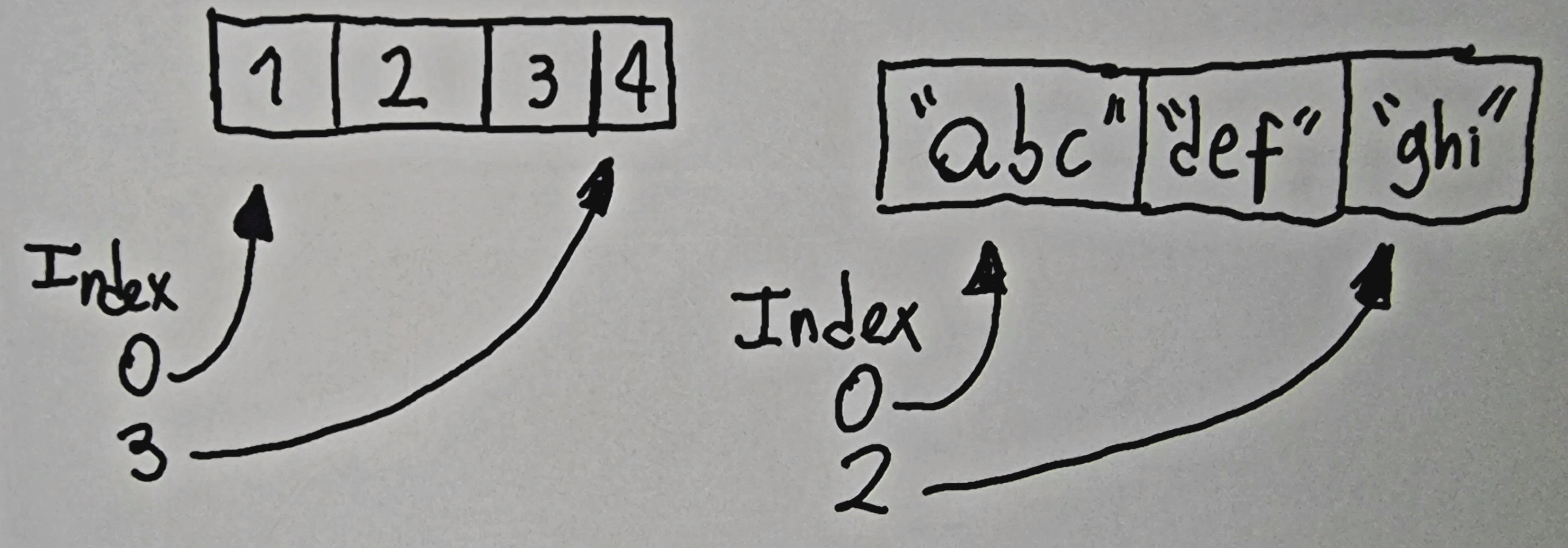
Creating arrays
The way to create arrays varies according to the programming language:
MY_ARRAY = ["A", "B", "C"] # array literal
my_array = list(range(5)) # array from range
When creating a literal array its elements are initialized directly. When constructing an empty array its size is specified but its elements are initialized with a default value (0 for numbers, null for objects, etc).
Accessing and modifying elements
Individual elements are quickly accessed by their index using brackets []:
my_array = ['a', 'b', 'c']
print(my_array[0]) # 'a'
print(my_array[2]) # 'c'
my_array[2] = 'z'
print(my_array[2]) # 'z'
Indices start at 0, so in an array of size N, valid indices are between 0 and N-1.
Accessing an invalid index causes an error, for example, accessing index 3 in an array of size 3. This is known as “index out of bounds”.
Traversing an array
We can traverse all elements using a for loop:
letters = ['a', 'b', 'c']

for i in range(len(letters)):
  print(letters[i])
This prints each element in order. len() returns the total length of the array.
Another way is by directly iterating over the elements:
letters = ['a', 'b', 'c']

for letter in letters:
  print(letter)
Searching in an array
We can search for an element in an array using a loop and comparing element by element:
letters = ['a', 'b', 'c']

def search_in_array(array, element):
  for i in range(len(array)):
    if array[i] == element:
      return i
  return False

print(search_in_array(letters, 'b')) # 1
print(search_in_array(letters, 'z')) # False
It returns the index if found or False if not found.
Multidimensional array
Arrays can have more than one dimension, for example, 2D matrices, 3D cubes, etc.
A 2D array can be seen as a table with rows and columns. To access an element two indices are specified, one for the row and one for the column:
matrix = [
  [1, 2, 3],
  [4, 5, 6]
]

print(matrix[0][2]) # 3
print(matrix[1][0]) # 4
They can have more dimensions, for example a 3D array to represent pixels in an image.
Conclusion
Arrays are fundamental data structures in programming that provide efficient access to elements in memory through numeric indices. Having a good command of arrays, matrices, and their uses is essential for any programmer.
Cheers for making it this far! I hope this journey through the programming universe has been as fascinating for you as it was for me to write down.
We’re keen to hear your thoughts, so don’t be shy – drop your comments, suggestions, and those bright ideas you’re bound to have.
Also, to delve deeper than these lines, take a stroll through the practical examples we’ve cooked up for you. You’ll find all the code and projects in our GitHub repository learn-software-engineering/examples.
Thanks for being part of this learning community. Keep coding and exploring new territories in this captivating world of software!
4.2 - Maps (Dictionaries)
A dictionary, or map, consists of a collection of key-value pairs. The key is used to access the associated value. Keys must be unique within a dictionary. Values can be repeated.
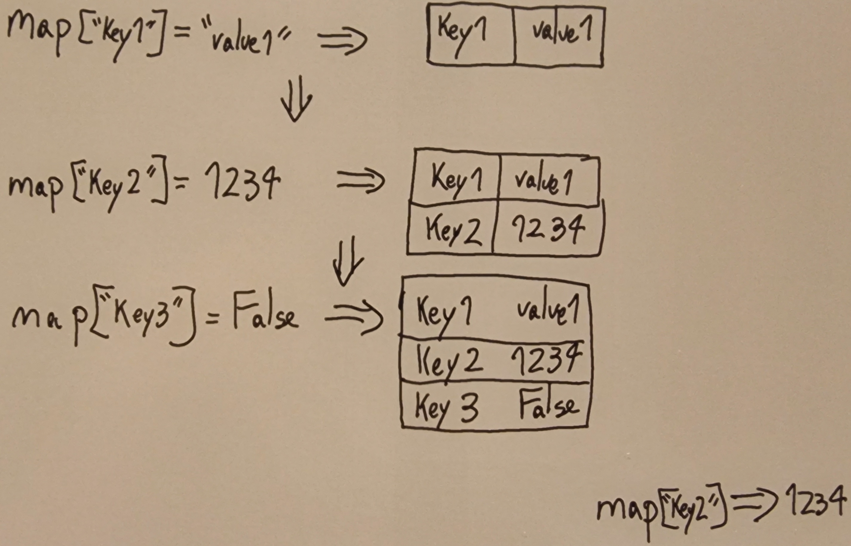
Main operations
- Add/update: Inserts a key-value pair. If the key existed, its value is replaced.
dictionary['key'] = 'value' - Get value: Accesses the value given a key.
value = dictionary['key'] - Delete: Removes a key-value pair from the dictionary.
del dictionary['key'] - Traverse: Iterate over the keys, values or pairs of the dictionary.
for key in dictionary:
  print(key, dictionary[key]) # key, value
Creating a dictionary or map
The syntax for creating maps or dictionaries in Python is:
empty_dictionary = {}

person = {
  'name': 'John',
  'age': 25
}
Usage examples
Dictionaries are useful in many cases. Below are some examples.
Objects and mappings
We can model objects and entities with key-value attributes:
product = {
  'name': 'Smartphone',
  'price': 500,
  'brand': 'XYZ'
}
Counts and frequencies
Counting occurrences of elements in sequences:
text = "Hello world world"

frequencies = {}

for word in text.split():
    if word in frequencies:
        frequencies[word] += 1
    else:
        frequencies[word] = 1

print(frequencies)
# {'Hello': 1, 'world': 2}
Storing and accessing data
As a high performance alternative to lists and arrays.
Conclusion
Dictionaries are versatile data structures thanks to their fast access based on unique keys. They have uses in almost all programs, so mastering dictionaries is essential in any language.
Cheers for making it this far! I hope this journey through the programming universe has been as fascinating for you as it was for me to write down.
We’re keen to hear your thoughts, so don’t be shy – drop your comments, suggestions, and those bright ideas you’re bound to have.
Also, to delve deeper than these lines, take a stroll through the practical examples we’ve cooked up for you. You’ll find all the code and projects in our GitHub repository learn-software-engineering/examples.
Thanks for being part of this learning community. Keep coding and exploring new territories in this captivating world of software!
4.3 - Linked Lists
A linked list is composed of nodes where each node has two parts:
- Data or information
- Reference to the next node
Nodes are organized sequentially, each pointing to the next. The last node points to null to indicate the end.
This dynamic structure allows efficient insertion and deletion of nodes.
Types of linked lists
There are several types:
- Singly linked: Each node points to the next one. Useful for queues and stacks.
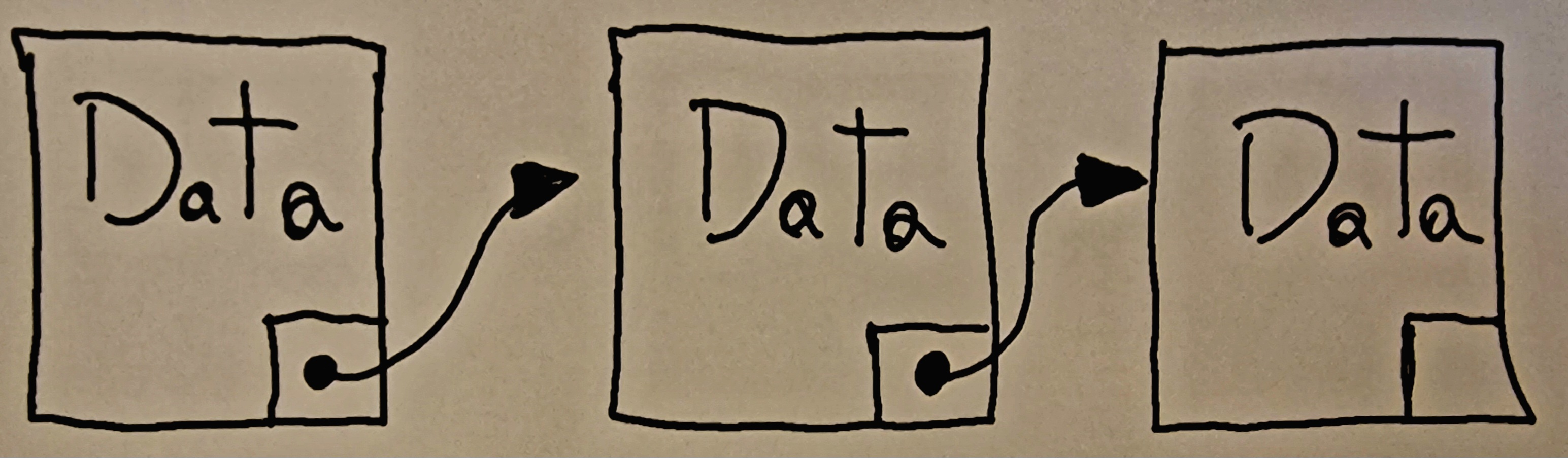
- Doubly linked: Each node has reference to the next and previous ones. Allows traversing in both directions.
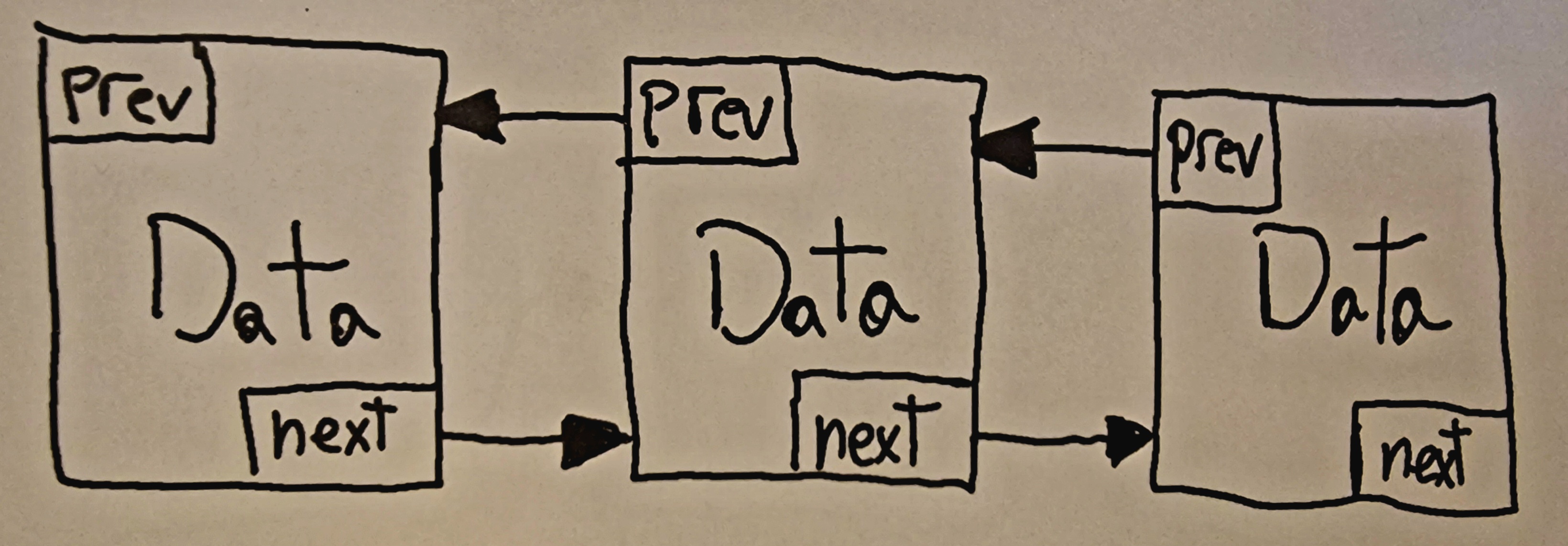
- Circular: The last node points to the first forming a cycle. Useful for circular buffers.

Common operations
Insert: Add nodes to the beginning, end or middle of the list.
Delete: Remove nodes by value or position.
Search: Find nodes by value by traversing the list.
Traverse: Iterate through nodes by following the references.
Implementation
Linked lists can be implemented as follows:
Use the ListNode class to represent nodes:
class ListNode:
  def __init__(self, value):
    self.value = value
    self.next = None
Then to create and use a list define a LinkedList class with methods for the operations:
class LinkedList:
  def __init__(self):
    self.head = None

  def add_to_start(self, new_value):
    new_node = ListNode(new_value)
    new_node.next = self.head
    self.head = new_node

  def print(self):
    current = self.head
    while current != None:
      print(current.value)
      current = current.next

  def search(self, searched_value):
    current = self.head
    while current != None:
      if current.value == searched_value:
        return True
      current = current.next
    return False

  #...other methods
With this LinkedList class we can create a list, add nodes, print it, search elements, etc.
We could add other methods like insert at end, delete by value, get by index, etc. But this gives an idea of how to encapsulate the linked list functionality in a class. As practice, feel free to try adding these methods on your own. Don’t hesitate to leave your comments and contact me if you need help!
Advantages and disadvantages
Advantages:
- Inserting and deleting nodes is efficient.
- Doesn’t require defining a fixed size like arrays.
- Dynamic, flexible structure.
Disadvantages:
- More memory usage from having to store references.
- Accessing elements by index is slower since it is sequential.
Usage examples
- Implementing structures like stacks and queues.
- In doubly linked lists, traverse the list in both directions.
- Blockchains like Bitcoin’s.
- Playing elements in order like music playlists.
Conclusion
Linked lists are a versatile data structure for storing dynamic sequences of elements. Having a good handle on these lists, their operations, and uses is essential for any programmer.
Cheers for making it this far! I hope this journey through the programming universe has been as fascinating for you as it was for me to write down.
We’re keen to hear your thoughts, so don’t be shy – drop your comments, suggestions, and those bright ideas you’re bound to have.
Also, to delve deeper than these lines, take a stroll through the practical examples we’ve cooked up for you. You’ll find all the code and projects in our GitHub repository learn-software-engineering/examples.
Thanks for being part of this learning community. Keep coding and exploring new territories in this captivating world of software!
4.4 - Stacks
The LIFO nature of stacks is due to the fact that only the top element can be accessed and manipulated. The operation of placing an element on the stack is known as “push”, while removing an element from the stack is a “pop”. The LIFO operation causes the last element placed in a stack to be the first to be removed.
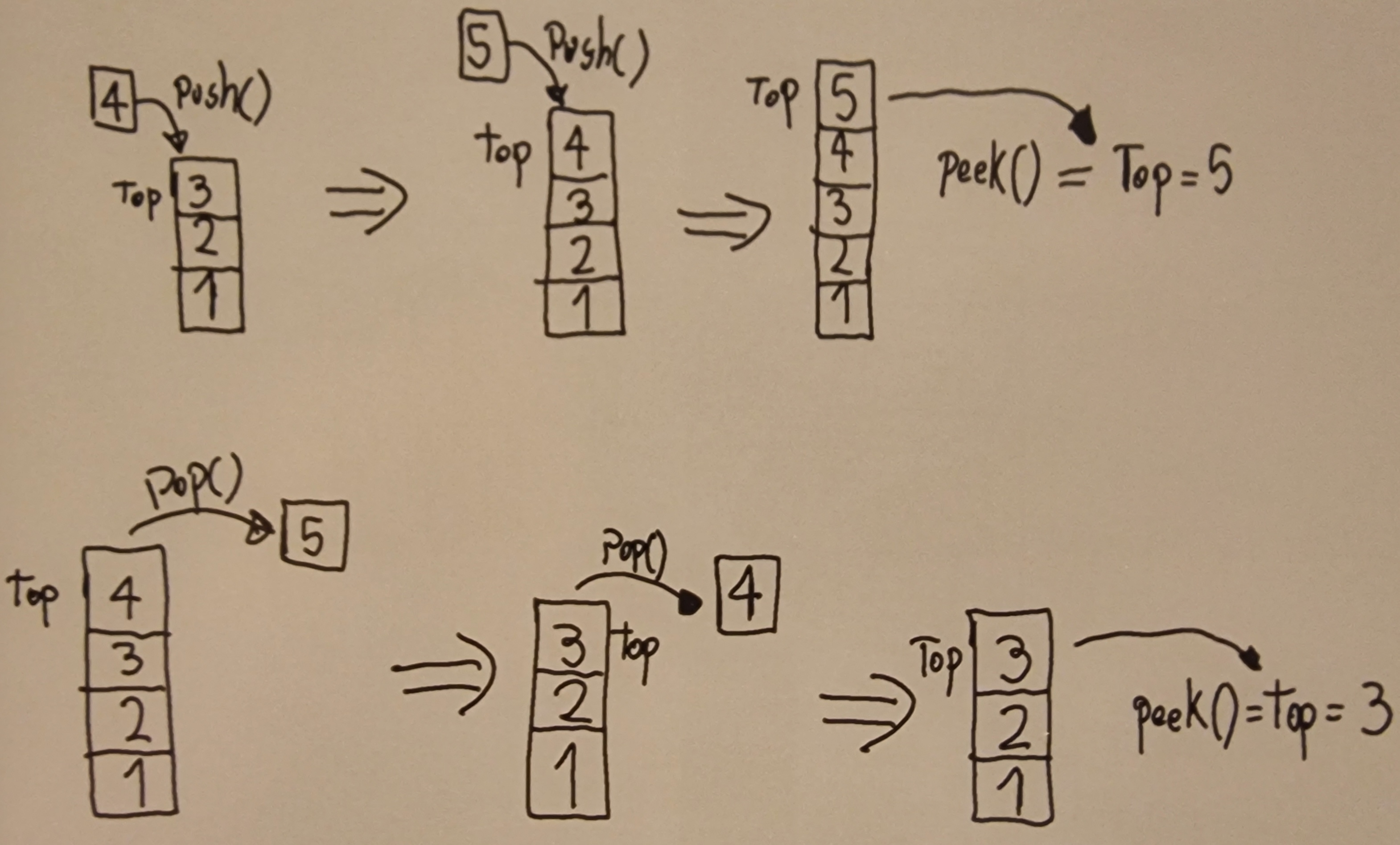
Main operations
The primary operations supported by a stack structure are:
- Push: adds an element to the top of the stack.
- Pop: removes the element at the top of the stack.
- Peek: allows accessing the top element without removing it from the stack.
- isEmpty: checks if the stack is empty.
Most languages like Python and Java provide stack implementations in their standard libraries.
Implementation
A stack can be implemented using a linked list so that each node points to the previous node.
class Node:
  def __init__(self, value):
    self.value = value
    self.previous = None


class Stack:
  def __init__(self):
    self.top = None
    self.size = 0

  def push(self, value):
    new_node = Node(value)
    if self.top is None:
      self.top = new_node
    else:
      new_node.previous = self.top
      self.top = new_node
    self.size += 1

  def pop(self):
    if self.top is None:
      return None
    top_node = self.top
    self.top = self.top.previous
    self.size -= 1
    return top_node.value

  def peek(self):
    if self.top is None:
      return None
    return self.top.value

  def is_empty(self):
    return self.top is None  # Returns true if top is None

  def __len__(self):
    return self.size

  def __str__(self):
    values = []
    current = self.top
    while current:
      values.append(str(current.value))
      current = current.previous
    return "\n".join(values)
Usage examples
Stacks have many uses in programming:
Execution stack (call stack): records pending function calls to resolve. Implements expected LIFO behaviour.
Browser stack: allows going back (undo) in the browser history similarly to a LIFO stack.
Math expression execution: stacks can verify parentheses, brackets, braces, etc.
Algorithms and data structures: like in the quicksort algorithm and in data path implementations.
Conclusion
Stacks are versatile data structures thanks to their LIFO operation principle. Having a good command of stacks, their uses and applications is essential in computer science.
Cheers for making it this far! I hope this journey through the programming universe has been as fascinating for you as it was for me to write down.
We’re keen to hear your thoughts, so don’t be shy – drop your comments, suggestions, and those bright ideas you’re bound to have.
Also, to delve deeper than these lines, take a stroll through the practical examples we’ve cooked up for you. You’ll find all the code and projects in our GitHub repository learn-software-engineering/examples.
Thanks for being part of this learning community. Keep coding and exploring new territories in this captivating world of software!
4.5 - Queues
The FIFO (first in, first out) nature of queues is because only the initial element can be accessed and manipulated. When an element is added to the queue it is known as “enqueue”, while removing an element is called “dequeue”.
This causes the first element to be added to the queue to also be the first to be removed, hence its FIFO behaviour.
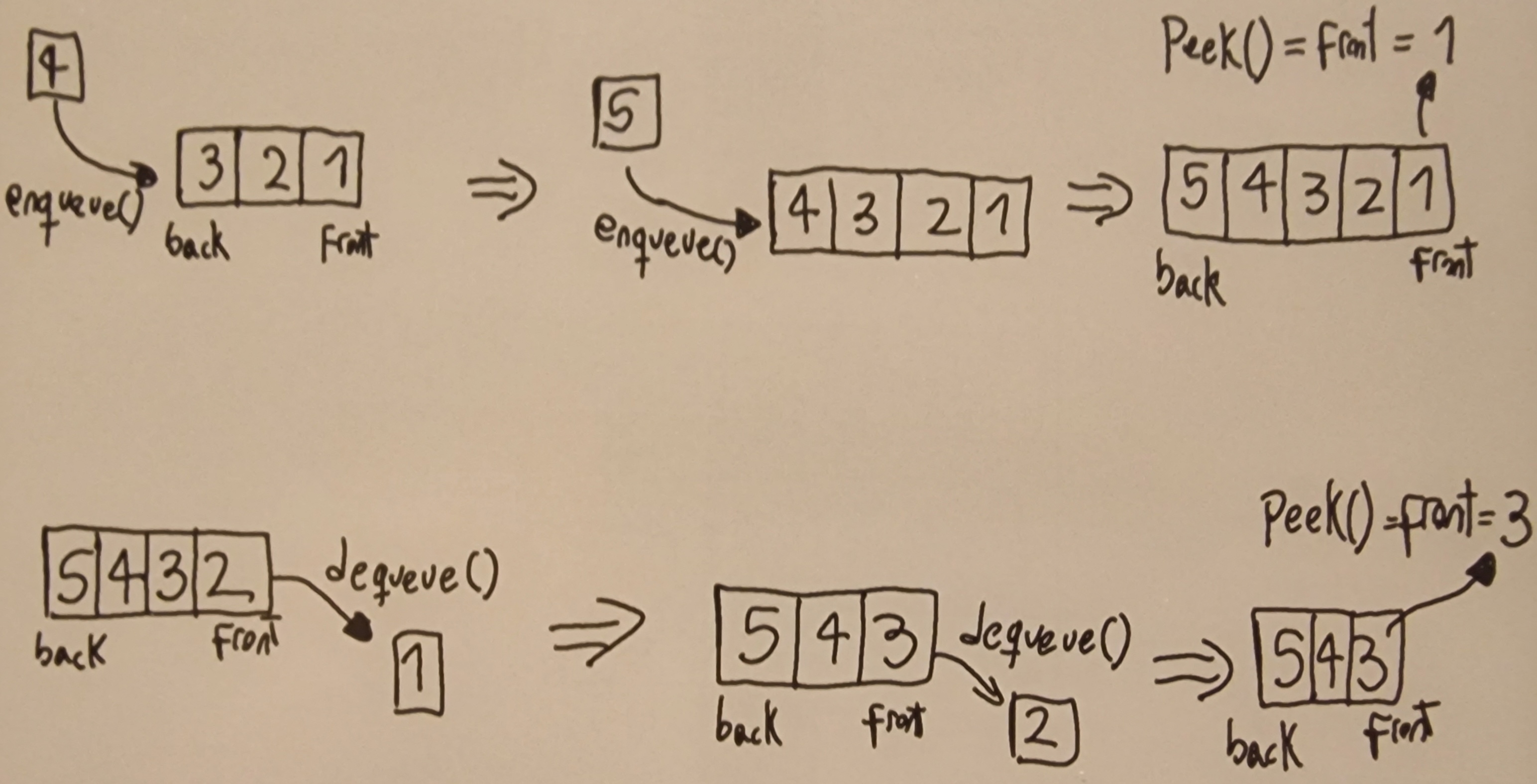
Main operations
The basic queue operations are:
- Enqueue: Adds an element to the end of the queue.
- Dequeue: Removes the element from the front of the queue.
- Peek: Gets the front element without removing it.
- isEmpty: Checks if the queue is empty.
Implementation
Like stacks, queues can be implemented using linked lists. Elements are added at the end and removed from the front by keeping references to both ends.
class Node:
  def __init__(self, value):
    self.value = value
    self.next = None


class Queue:
  def __init__(self):
    self.front = None
    self.end = None
    self.size = 0

  def enqueue(self, value):
    new_node = Node(value)
    if self.end is None:
      self.end = new_node
      self.front = new_node
      return
    self.end.next = new_node
    self.end = new_node
    self.size += 1

  def dequeue(self):
    if self.is_empty():
      return None
    value = self.front.value
    self.front = self.front.next
    if self.front is None:
      self.end = None
    self.size -= 1
    return value

  def peek(self):
    if self.is_empty():
      return None
    return self.front.value

  def is_empty(self):
    return self.front is None  # Returns true if front is None

  def __len__(self):
    return self.size

  def __str__(self):
    values = []
    current = self.front
    while current:
      values.append(str(current.value))
      current = current.next
    return "\n".join(values)
Usage examples
Some common uses of queues:
- Print queues where first in, first printed.
- Task queues in operating systems for execution order.
- Simulations where arrival order must be respected like in banks.
- Message queues like RabbitMQ or Kafka.
- Circular buffers in audio for streaming.
Conclusion
Queues are versatile structures thanks to their FIFO principle. Having a good handle on queues, implementation, and applications will reinforce your skills as a programmer.
Cheers for making it this far! I hope this journey through the programming universe has been as fascinating for you as it was for me to write down.
We’re keen to hear your thoughts, so don’t be shy – drop your comments, suggestions, and those bright ideas you’re bound to have.
Also, to delve deeper than these lines, take a stroll through the practical examples we’ve cooked up for you. You’ll find all the code and projects in our GitHub repository learn-software-engineering/examples.
Thanks for being part of this learning community. Keep coding and exploring new territories in this captivating world of software!